While working in Excel there can be some duplicate rows in your worksheet, and then you may want to find or highlight the duplicate rows because the duplicate rows can create a lot of trouble. In this article, you will learn 5 easy methods to find duplicate rows in Excel.
This is an overview of this article.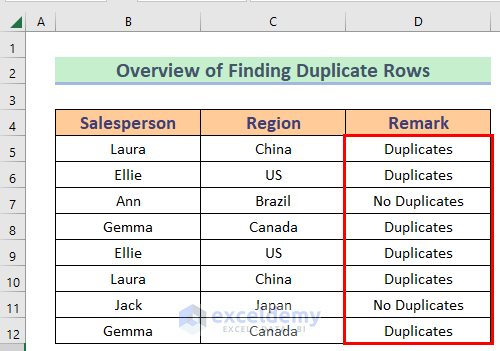
How to Find Duplicate Rows in Excel: 5 Quick Ways
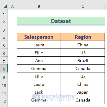
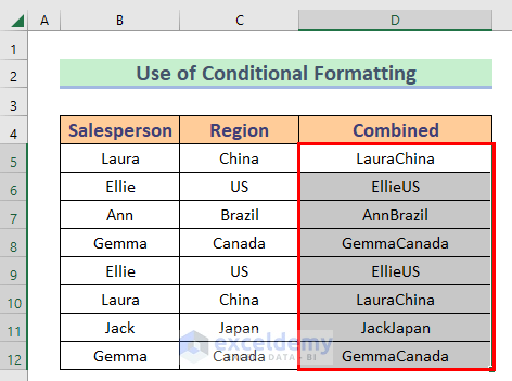
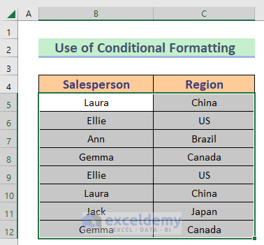
Let’s get introduced to our dataset first. I have used some salespersons’ names and their corresponding regions in our dataset. Please have a look that there are some duplicate rows in the dataset.
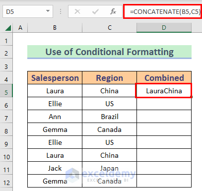
Method 1: Use CONCATENATE Function and Conditional Formatting to Find Duplicate Rows in Excel
First of all, I will use the CONCATENATE function and Conditional Formatting to find duplicate rows in Excel. The CONCATENATE function is used to join two or more strings into one string.
Steps:
- At first, we’ll combine the data from every row. That’s why I have added a new column named “Combined” to apply the CONCATENATE function.
- Type the formula given below-
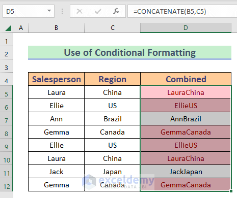
=CONCATENATE(B5,C5)
- Then hit the Enter button to get the output.
- After that, use Fill Handle to AutoFill up to D12.
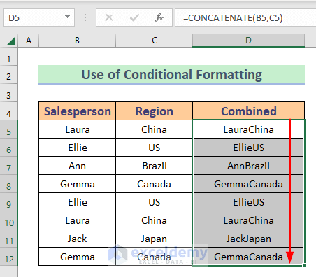
- After that, select D5:D12.
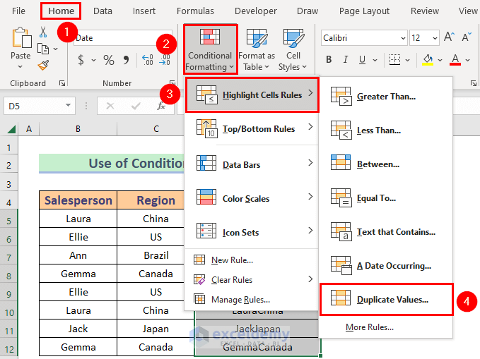
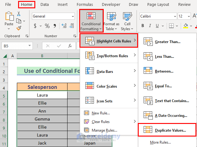
- Then, go to Home tab.
- After that, select Conditional Formatting.
- Following that, select Highlight Cell Rules.
- Finally, select Duplicate Values.
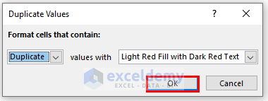
- A box will appear. Click OK.
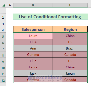
- Excel will highlight the duplicate rows.
Read more: How to Find Repeated Cells in Excel
Method 2: Apply Conditional Formatting
In this method, we’ll again use Conditional Formatting. This method is a bit easier because it will not need any helper column like the previous method.
Steps:
- Select B5:C12.
- Then, go to the Home tab.
- After that, select Conditional Formatting.
- Following that, select Highlight Cell Rules.
- Finally, select Duplicate Values.
- A box will appear. Click OK.

- Excel will highlight the duplicate rows.
Read more: How to Find Repeated Numbers in Excel
Method 3: Insert COUNTIF Function to Find Matched Rows in Excel
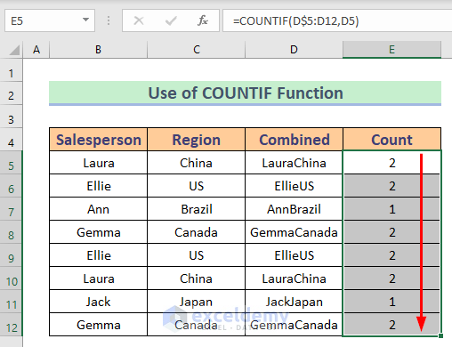
Here we’ll use only the COUNTIF function to find duplicate rows in Excel. The COUNTIF function will count the duplicate numbers and then from that, we’ll be able to detect the duplicate rows. I have added another column named “Count”.
Steps:
- Activate Cell E5.
- Then, type the given formula
=COUNTIF(D$5:D12,D5)
- After that, press ENTER to get the output.
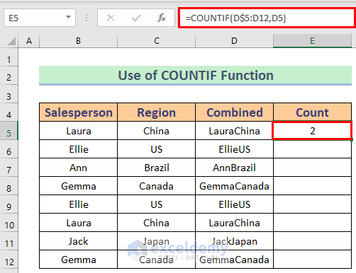
Here, Excel will count the instances if the rows are duplicates in the range D5:D12.
- After that, use Fill Handle to AutoFill up to D12.
Read More: How to Filter Duplicates in Excel
Method 4: Combine IF Function and COUNTIF Function to Find Replica Rows in Excel
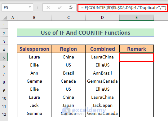
In this method, we’ll combine the IF function and the COUNTIF function to find duplicate rows in Excel. The IF function checks whether a condition is met and returns one value if true and another value if false.
Steps:
- In Cell E5 write the given formula.
=IF(COUNTIF($D$5:$D5,D5)>1,"Duplicate","")
- Then press ENTER to get the output.
Formula Explanation
- COUNTIF($D$5:$D5,D5)>1 → This is the logical test. It will be TRUE if a duplicate row appears.
- Output: FALSE
- IF(COUNTIF($D$5:$D5,D5)>1,”Duplicate”,””) → This becomes,
- IF(FALSE,”Duplicate”,””)
- Output: “” (blank)
- After that, use Fill Handle to AutoFill up to E12.
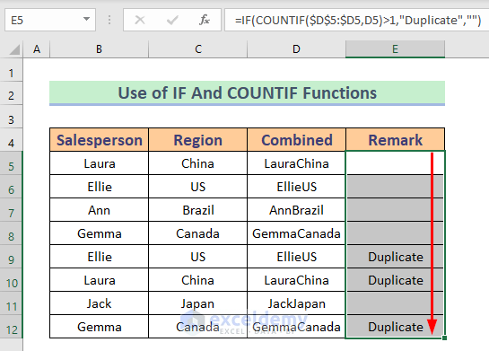
The difference between this method with the previous ones is that here the 1st instance of a row is not considered a duplicate one.
Read More: How to Compare Rows for Duplicates in Excel
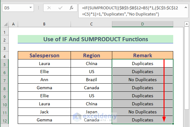
Method 5: Use IF Function and SUMPRODUCT Function Together to Find Duplicate Rows in Excel
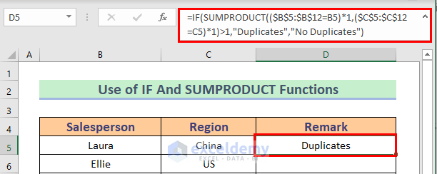
In our last method, we’ll use another combination of two functions- the IF function and the SUMPRODUCT function. The SUMPRODUCT is a function that multiplies the range of cells or arrays and returns the sum of products.
Steps:
- Write the combined formula in Cell D5.
=IF(SUMPRODUCT(($B$5:$B$12=B5)*1,($C$5:$C$12=C5)*1)>1,"Duplicates","No Duplicates")
- Then, press ENTER to get the output.
Formula Breakdown
- SUMPRODUCT(($B$5:$B$12=B5)*1,($C$5:$C$12=C5)*1)>1 → The SUMPRODUCT function will check the array whether it is greater than 1 or not. Then it will show TRUE for greater than 1 otherwise FALSE. It will return as-
- Output: {TRUE}
- IF(SUMPRODUCT(($B$5:$B$12=B5)*1,($C$5:$C$12=C5)*1)>1,”Duplicates”,”No Duplicates”) → Then the IF function will show “Duplicates” for TRUE and “No duplicates” for FALSE. The result will be-
- Output: {Duplicates}
- After that, use Fill Handle to AutoFill up to D12.
Read More: Excel Find Duplicate Rows Based on Multiple Columns
Download Practice Workbook
You can download the free Excel template from here and practice on your own.
Conclusion
I hope all of the methods described above will be good enough to find duplicate rows in excel. Feel free to ask any questions in the comment section and please give me feedback.
Related Articles
- How to Compare Two Excel Sheets for Duplicates
- How to Find Matching Values in Two Worksheets in Excel
- How to Find Duplicates in Excel and Copy to Another Sheet
- Excel VBA to Find Duplicate Values in Range
- How to Find Duplicates in a Column Using Excel VBA
- How to Use VBA Code to Find Duplicate Rows in Excel
<< Go Back to Find Duplicates in Excel | Duplicates in Excel | Learn Excel
Get FREE Advanced Excel Exercises with Solutions!

Is there a formula to find duplicates (Laura & China and China & Laura) if table was like this:
Salesperson Region
Laura China
Ellie US
Ann Brazil
China Laura
Gemma Canada
US Ellie
Hello YVONNE
Thanks for reaching out and sharing your query. You wanted a formula to find duplicates when columns can be suffered, like Laura & China and China & Laura.
I have developed two formulas that will fulfil your requirements using the IF and COUNTIF functions. I will use column C as a Helper column, displaying the result in column D.
Follow these steps:
Step 1: Select cell D5 => Insert the given formula => Drag the Fill Handle icon to cell D10.
Step 2: Select cell D5 => Insert the given formula => Drag the Fill Handle icon to cell D10.
Hopefully, you have got the solution. Good luck.
Regards
Lutfor Rahman Shimanto