Hyperlink means to create a link between two or more data. It takes you to the detailed data whenever you click on the link. You can connect your data or cells within the same sheet or to another worksheet. Excel provides you with several methods to create hyperlinks to cells. You can also create a dynamic hyperlink to your cell. In this article, we discussed methods for creating a hyperlink to a cell in Excel. So, let’s get started.
How to Hyperlink to Cell in Excel: 4 Methods
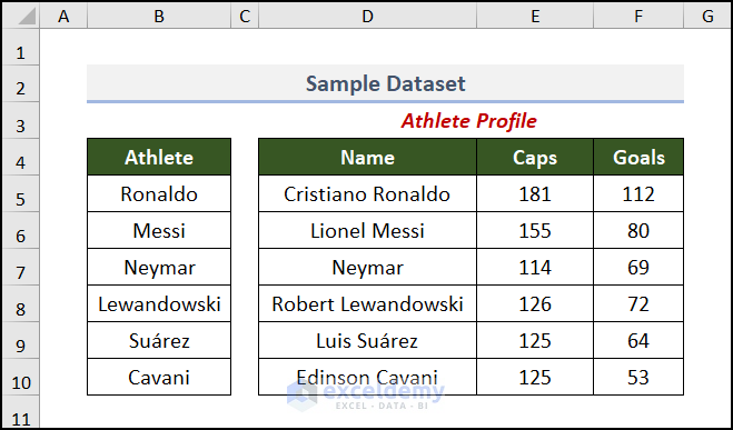
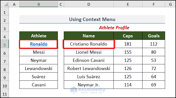
For hyperlinking your cell data to the same sheet or another sheet, you have to create a dataset first. We have included some famous Athlete names in the Athlete Profile. Now, we will hyperlink to a cell with this dataset.
Not to mention, we have used the Microsoft 365 version. You can use any other version at your convenience.
1. Using the Link Option from Context Menu
You can link up with the same dataset using the Context Menu. It is an easy and straightforward method. All you need to do is link up the data with another cell. Follow the procedure.
Steps:
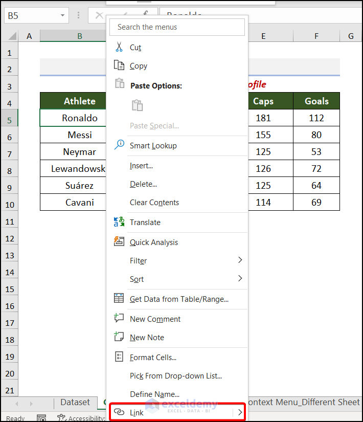
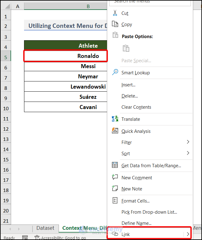
- Firstly, right-click the cell that you want to hyperlink.
- Apparently, the Context Menu appears. Click on the Link.
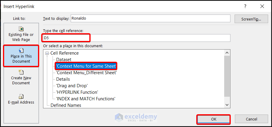
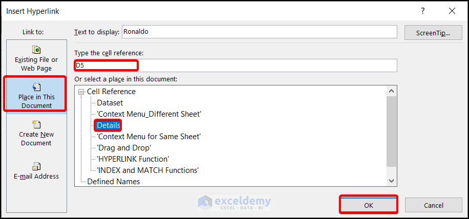
- Consequently, an Insert Hyperlink dialog box appears. Move to the Place in the Document to the Link to section. Choose the cell reference D5 in the Type the cell reference box. In the Cell Reference box select the sheet that you want to link up.
- Finally, hit OK.
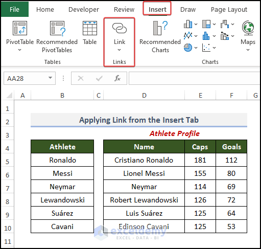
Note: Also, you can pick the Link option from the Links groups of the Insert tab.
Similarly, pressing CTRL + K will bring up the Insert Hyperlinks window.
Your link has been created with the blue sign. It refers to the D5 cell, as we linked it to that.
Similarly, apply the same procedure for all other cells, and you will have hyperlinked all the cells like the gif below.
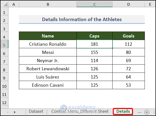
Additionally, you can perform it for different sheets as well. For completing the operation, you need to create a different sheet with the Athlete Profile. In our case, we set the sheet name as “Details”.
- Initially, right-click on the cell that you want to link up and choose Link from the Context Menu.
- Sequentially, in the Insert hyperlink window choose the Type the cell reference. And in the Cell Reference box click on the Details (the sheet name). Hit OK.
- You can see the hyperlink has been created in the selected cell.
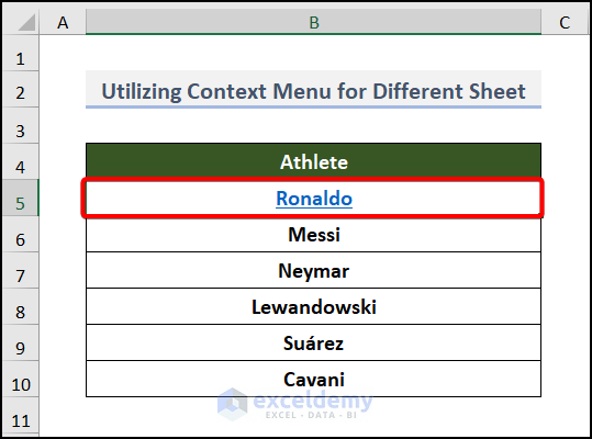
Eventually, when you click on the link, it will take you to the sheet that you hyperlinked (see the below gif).
Read More: How to Hyperlink to Cell in Same Sheet in Excel
2. Utilizing Cell Dragging and Dropping
It is a very simple method to create a hyperlink to a cell where you have to just drag and drop your cursor.
Steps:
- First, just drag the source data cell to the cell where you want to create the hyperlink. At the same time, you have to right-click.
- Following that, release the mouse and you will see the Context Menu. Choose the Create Hyperlink Here option.

See the below gif for better visualization.

Similarly, you can repeat the same thing for other cells and get the result like the image below.
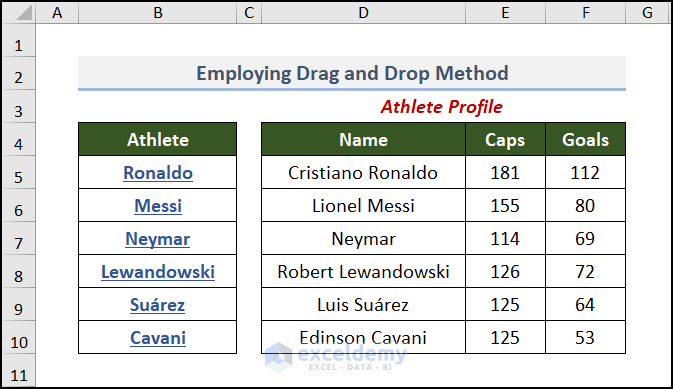
You can also create hyperlinks to another sheet by the cell drag and drop method.
Read More: Excel Hyperlink to Cell in Another Sheet with VLOOKUP
3. Applying the HYPERLINK Function
Excel provides you with a function for creating hyperlinks. The HYPERLINK function basically creates links with the same or another sheet. Here, we have discussed it for the different sheets, but you can also use the formula for creating hyperlinks to the same sheet. Follow the below instructions to use the function.
Steps:
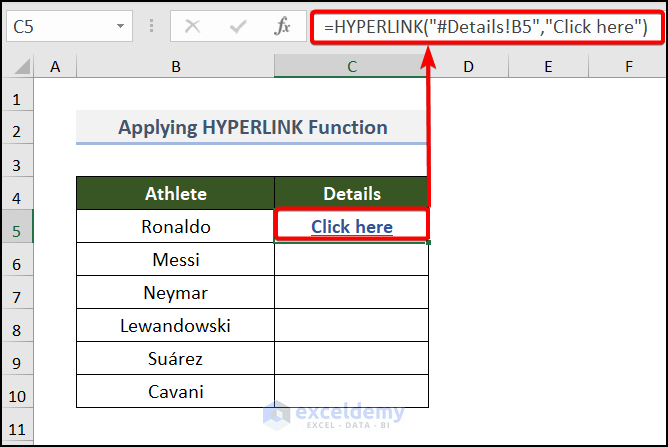
- Firstly, go to cell C5 where you want to create the hyperlinks.
- Secondly, insert the below formula.
=HYPERLINK("#Details!B5","Click here")The HYPERLINK function returns a clickable value. Here, we’ll get the link to cell B5. Furthermore, we’ve used a hash (“#”) to indicate the sheet “Details.” Then, we’ll display the second part in cell C5 of another sheet and make the text “Click here”. Whenever you click on the text “Click here”, it redirects you to the linked sheet (Details).
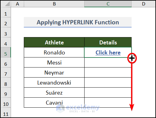
- Eventually, press ENTER and drag down the Fill Handle tool for the other cells.
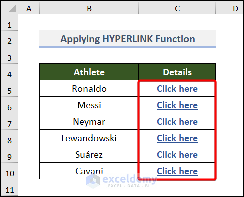
Finally, all the cells are filled with the text “Click here”.
Here, we have added a gif for a better understanding.
Read More: How to Hyperlink Multiple Cells in Excel
4. Adding Dynamic Hyperlink
You can create a dynamic hyperlink with some of the combined functions. Here, we have used the CELL, the INDEX, and the MATCH functions together to find a specific value on different sheets. But you can apply the formula to the same sheet as well. Go through the below steps to get a proper idea.
Steps:
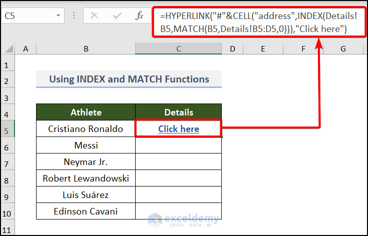
- Firstly, move to cell C5 and input the formula.
=HYPERLINK("#"&CELL("address",INDEX(Details!B5,MATCH(B5,Details!B5:D5,0))),"Click here")Formula Breakdown
- MATCH(B5, Details!B5:D5,0)→The MATCH function is used to find the position of a value. Here, we’re looking for the value B5 (Cristiano Ronaldo) in the sheet and range Details!B5:D5. Moreover, we’ve put the 0 for exact matching.
- Output:
- INDEX(Details!B5,MATCH(B5,Details!B5:D5,0))→The INDEX function returns a value from a range. Here, we’re getting the value from the MATCH function and the data range is B5:D5.
- Output: “Cristiano Ronaldo”.
- Then our formula in the CELL portion reduces to, CELL(“address”,” Details!$B$5”)→The CELL function returns information about a cell. Here, we’ve set out info_type as “address”. This will return the first occurrence of the text “Cristiano Ronaldo” in our range which is in sheet Details!$B$5.
- HYPERLINK(“#”&CELL(“address”,INDEX(Details!B5,MATCH(B5,Details!B5:D5,0))),”Click here”)→The HYPERLINK function returns a clickable value. Here, we’ll get the link to cell B5. Moreover, we’ve put a hash (“#”) to indicate within the sheet named Details. Then, we’ll display the second part in cell C5 of another sheet and make the text “Click here”. Whenever you click on the text Click here, it redirects you to the linked sheet (Details).
- Output: “Click here”.
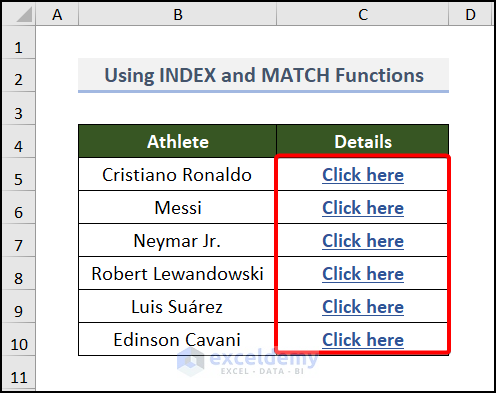
Finally, press ENTER and drag it down for the other cells to get the below result.
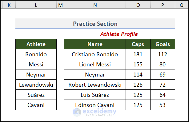
Practice Section
We have provided a practice section on each sheet on the right side for your practice. Please do it by yourself.
Download Practice Workbook
Download the following practice workbook. It will help you to realize the topic more clearly.
Conclusion
That’s all about today’s session. These are some easy methods for creating a hyperlink to a cell in Excel. Please let us know in the comments section if you have any questions or suggestions. For a better understanding, please download the practice sheet. Thanks for your patience in reading this article.
Further Readings
- How to Create a Hyperlink in Excel
- How to Activate Multiple Hyperlinks in Excel
- Excel Hyperlink with Shortcut Key
- How to Link a Website to an Excel Sheet
- How to Fix Broken Hyperlinks in Excel
- How to Hyperlink Multiple PDF Files in Excel
- How to Link Files in Excel
- How to Create Button Without Macro in Excel
<< Go Back To Create Hyperlink in Excel | Hyperlink in Excel | Linking in Excel | Learn Excel
Get FREE Advanced Excel Exercises with Solutions!
