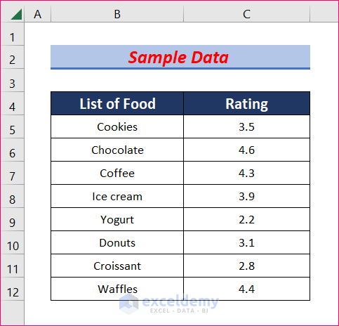
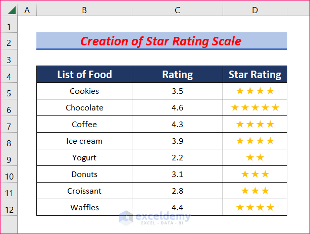
We will use the following dataset to demonstrate how to make a rating scale. It has a number of products and a rating score for each of them.
Method 1 – Use Conditional Formatting to Create a Star Rating Scale in Excel
Steps:
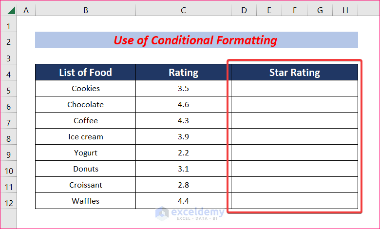
- Insert five helper (result) columns named Star Rating beside the Rating column. Remove the borders between them.
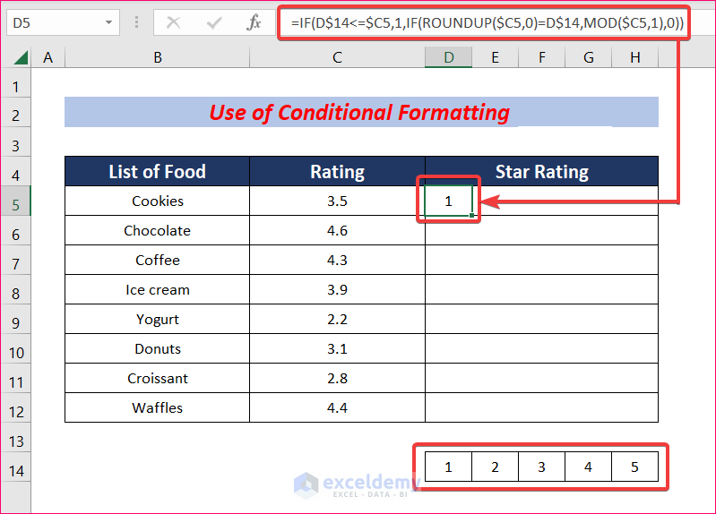
- Write 1 to 5 in cells D14 to H14.
- Select cell D5 and copy the following formula into it:
=IF(D$14<=$C5,1,IF(ROUNDUP($C5,0)=D$14,MOD($C5,1),0))Formula Breakdown:
- MOD($C5,1) returns the remainder after dividing cell C5 by 1.
- IF(ROUNDUP($C5,0)=D$14) rounds up the C5 cell value to 1.
- IF(D$14<=$C5,1,IF(ROUNDUP($C5,0)=D$14,MOD($C5,1),0)) returns 1 if C5>D14 and returns the decimal part if C5<D14.
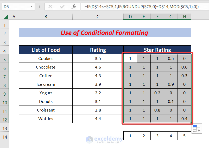
- Autofill the formula to the rest of the cells across columns and rows.
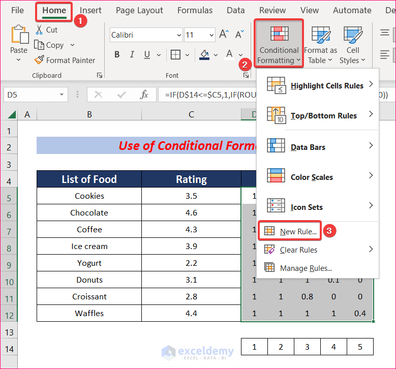
- From the Home tab, go to Conditional Formatting and select New Rule.
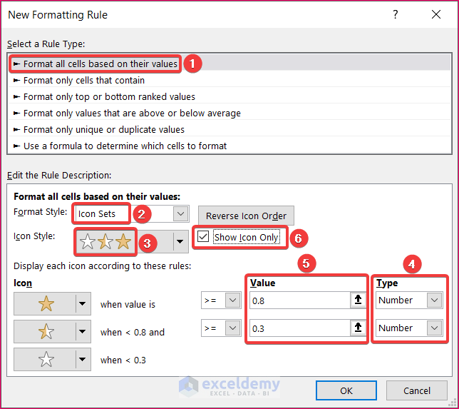
- A New Formatting Rule dialogue box will appear. Select Format all cells based on their values.
- Choose Icon Sets in the Format Style option.
- Select 3 Stars as the Icon Style.
- Change the Type to Number.
- Set values to show a filled star, half-filled star, or empty star. We set values 8 and 0.3 in this example. Any value less than 0.3 will show an empty star, a value between 0.3 to 0.8 will show a half-filled star and a filled star will be visible if the value is greater than 0.8.
- Check the box for Show Icon Only and press Enter.
- You will find star ratings for all the food items.
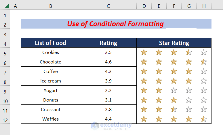
- You can change any of the food ratings and the star rating will automatically get updated.
Read More: How to Make Yes Green and No Red in Excel
Method 2 – Apply the REPT Function
Case 2.1 – Add Data Bars to Create a Rating Scale
Steps:
- Insert a column D named Bar Rating.
- Select cell D5 and copy the following formula there:
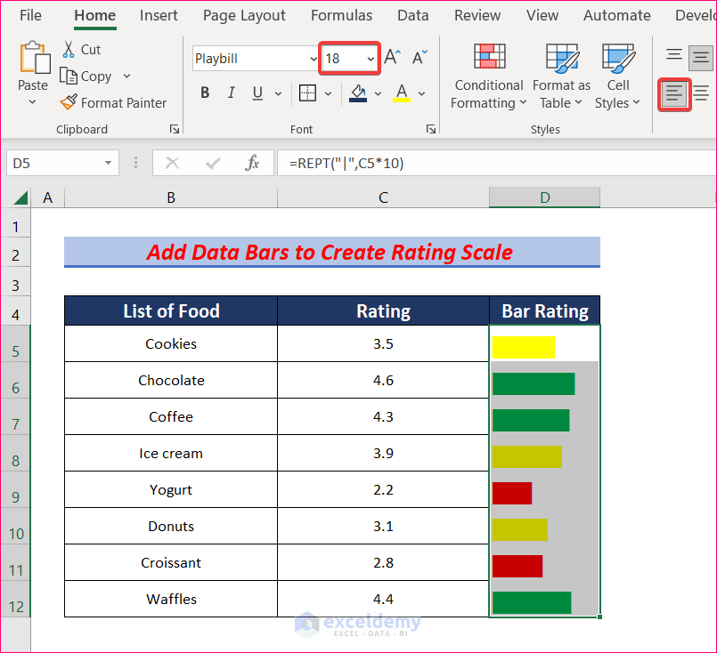
=REPT("|",C5*10)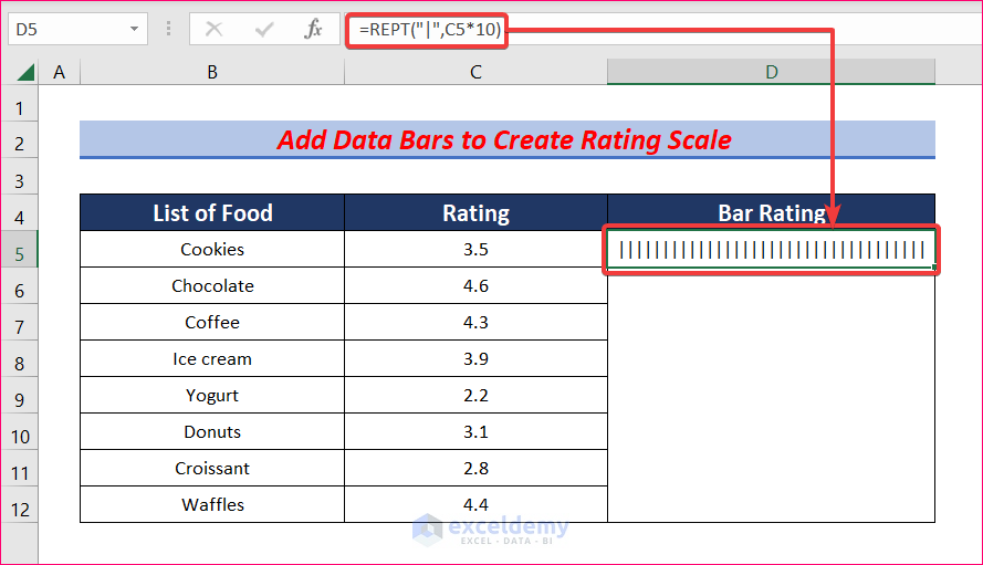
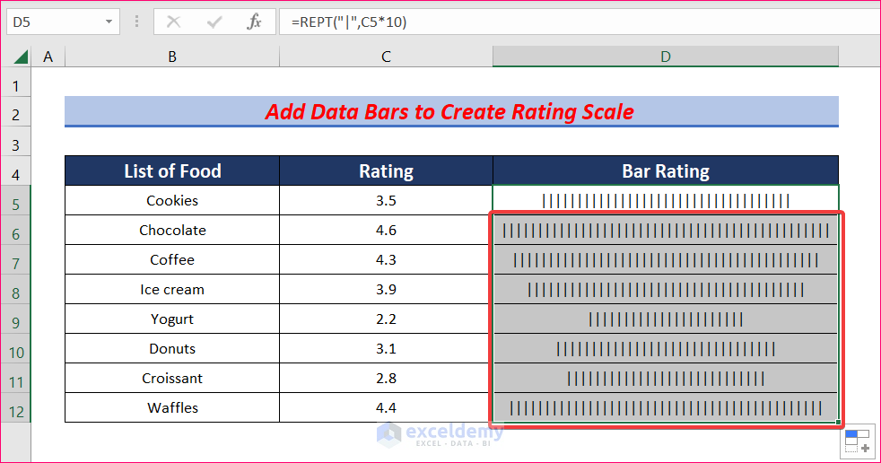
- Autofill the formula to the rest of the cells in column D.
- Select the D column with all the vertical bars and change the text font to Playbill.
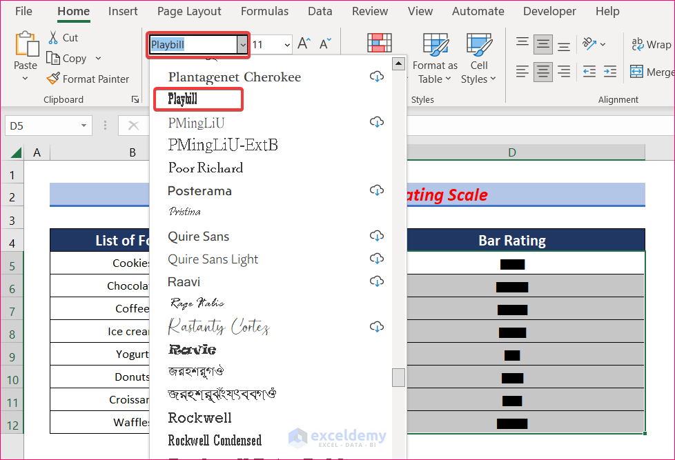
- The vertical bars will look like one single wide bar.
- Select column D and from the Home tab, go to Conditional Formatting and pick New Rule.
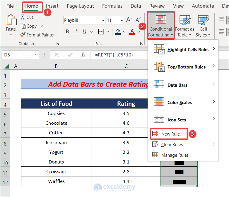
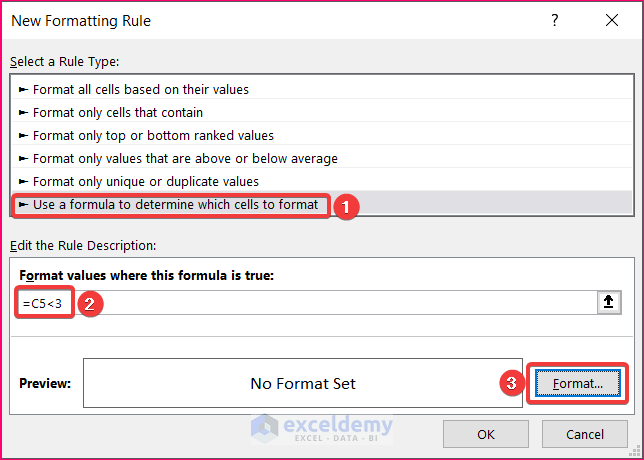
- Select Use a formula to determine which cells to format and insert the following formula.
=C5<3- Go to Format.
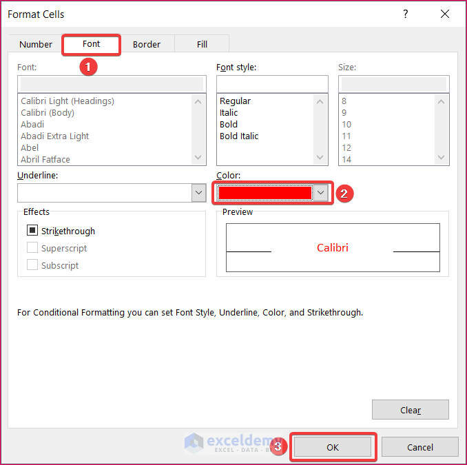
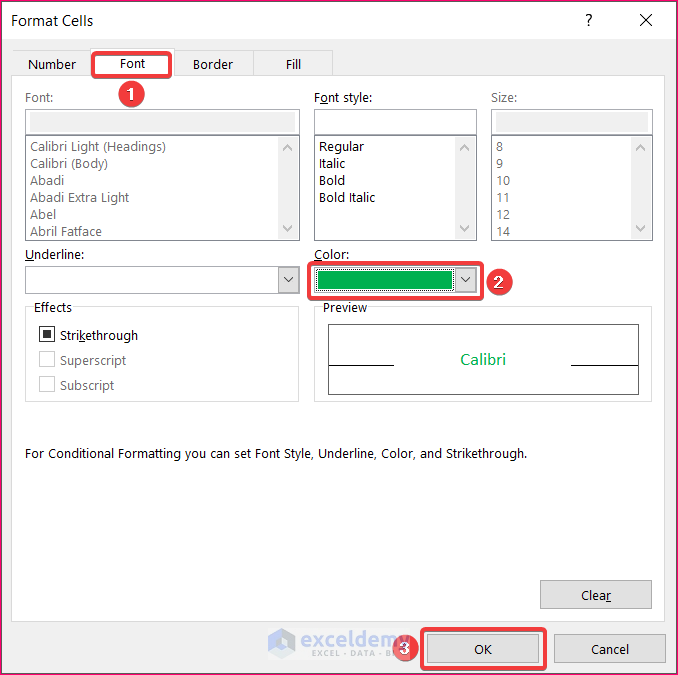
- In the Format Cells box, go to the Font tab and change the Color to Red.
- Click OK.
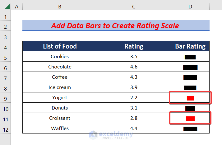
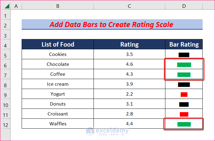
- The bars with ratings lower than 3 will be turned into red.
- Insert a New Conditional Formatting Rule with the following formula in the New Format Cells dialogue box.
=C5>4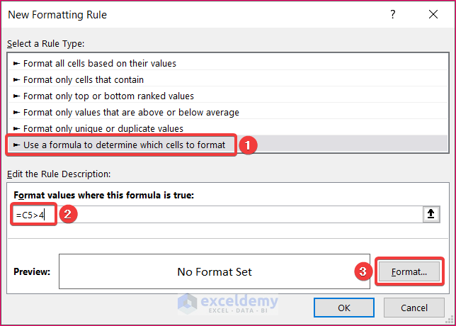
- Select the color Green from the Font tab.
- The bars that represent a rating higher than 4 will turn green.
- Follow the same process to apply the yellow formatting color for values between 3 and 4.
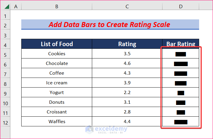
- Increase the font size of the bars and align them to the left.
2.2 – Create a Star Rating Scale
Steps:
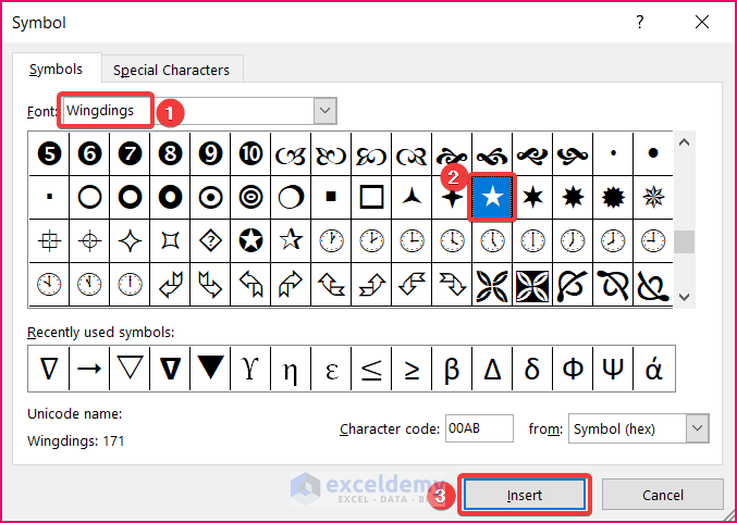
- Select any cell and then go to Insert, then to Symbols, and pick Symbol.
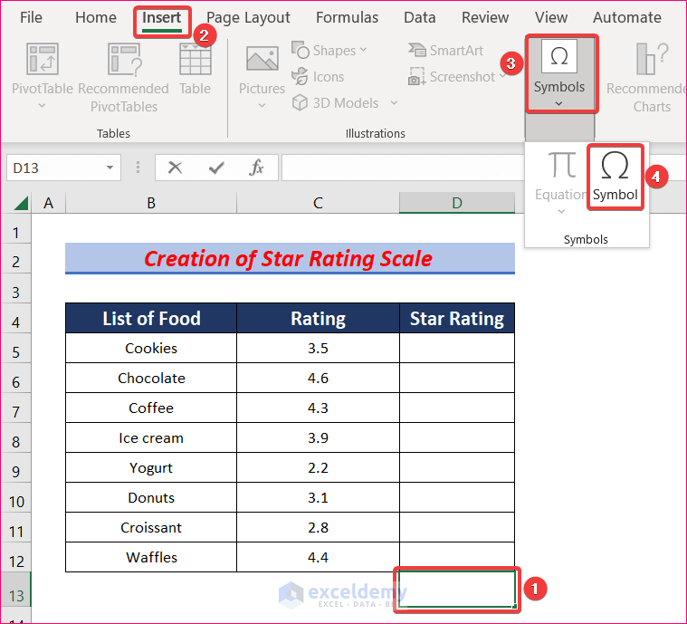
- From the Wingdings font, insert the Star symbol.
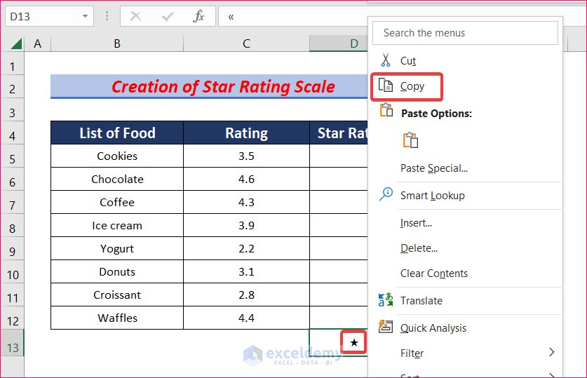
- Copy the star symbol.
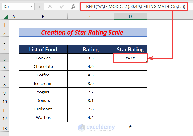
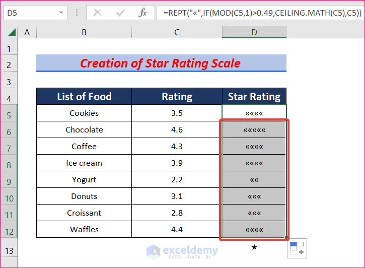
- Select cell D5 and copy the following formula there. Paste the copied star between “”.
=REPT("«",IF(MOD(C5,1)>0.49,CEILING.MATH(C5),C5))Formula Breakdown:
- CEILING.MATH(C5) rounds up the C5 cell value to the next integer.
- MOD(C5,1)>0.49 checks if the remainder of cell C5 divided by 1 is greater than 49 or not.
- Autofill the formula to the rest of the cells in column D.
- To convert the “<<” symbol to the Star symbol, select column D and change the font to Wingdings.
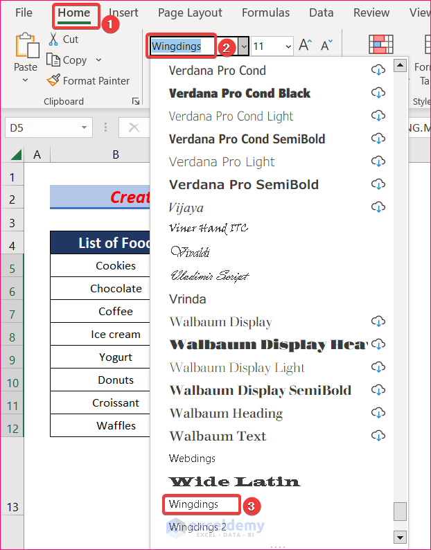
- You will find that all the symbols have now turned into stars.
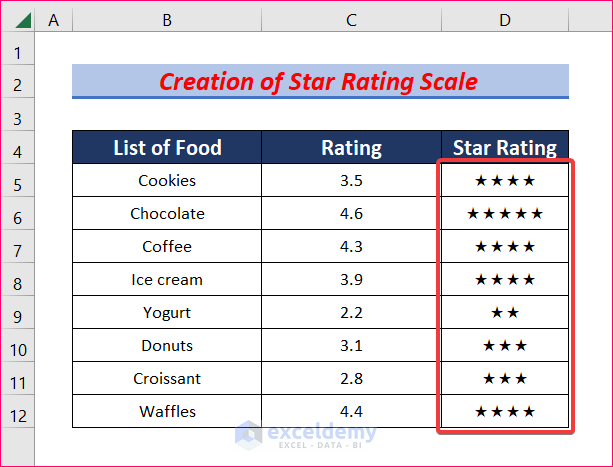
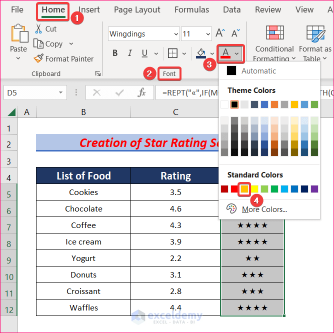
- Change the font and color of the symbols to enhance their appearance.
- You will get your desired rating scale.
Read More: How to Apply Borders in Excel with Conditional Formatting
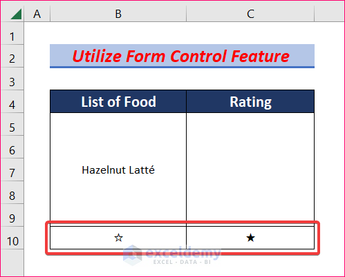
Method 3 – Use the Form Control Feature to Create a Star Rating Scale
Now we will use the Form Control feature to create a star rating scale in Excel. The procedure is discussed in the following section.
Steps:
- First copy these two symbols (☆★) from here and paste them into two different cells.
- Next, go to the Developer tab, and from there,
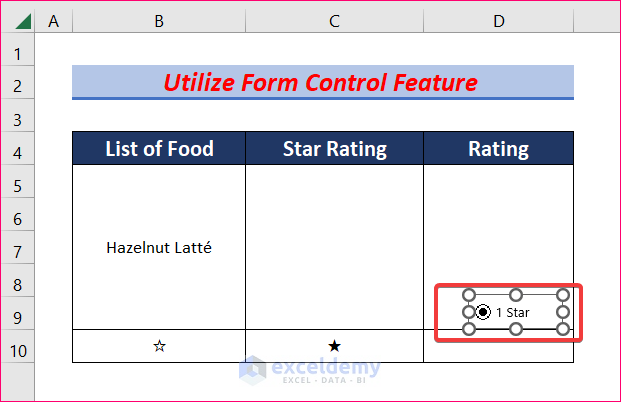
Developer → Insert → Form Control → Option Button
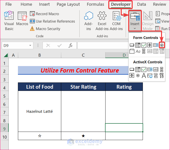
- Click and drag your cursor to insert the Option button in cell D9.
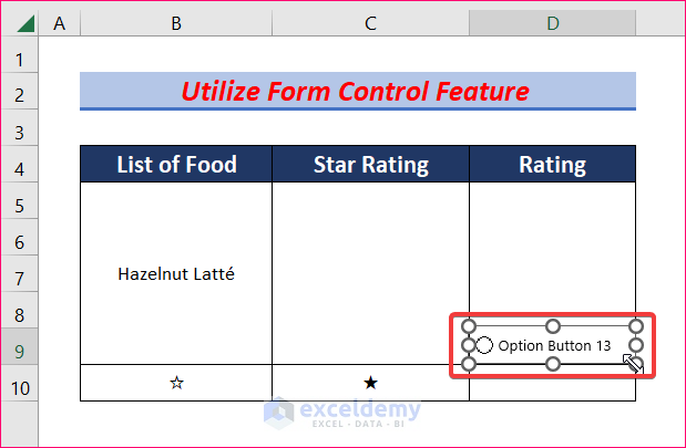
- Then double-click on the text to edit the text beside the button.
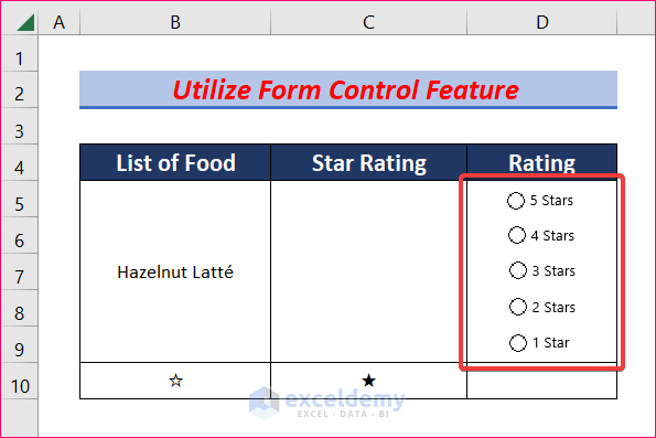
- Similarly, add four more buttons to cells D8 to D5.
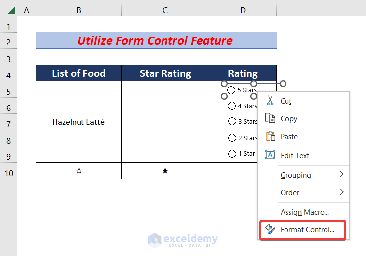
- Now right-click on any of the buttons and select Format Control.
- The Format Control box will pop up.
- In the box, go to the Control tab and select Unchecked.
- Then choose cell D10 to link the buttons.
- After that, click Ok.

- Next, write down the following formula in the Star Rating column.
=REPT(B10,5-D10)&REPT(C10,D10)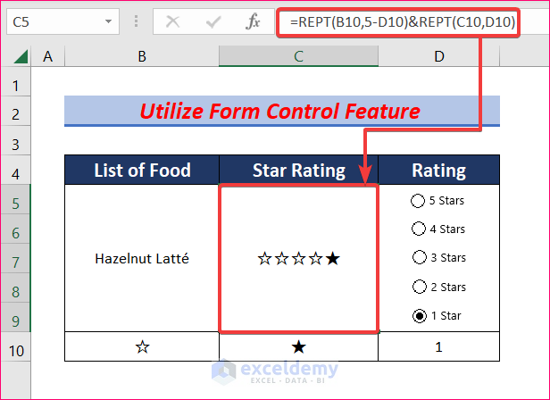
- Then from the Home tab, go to,
Home → Alignment → Orientation → Vertical Text
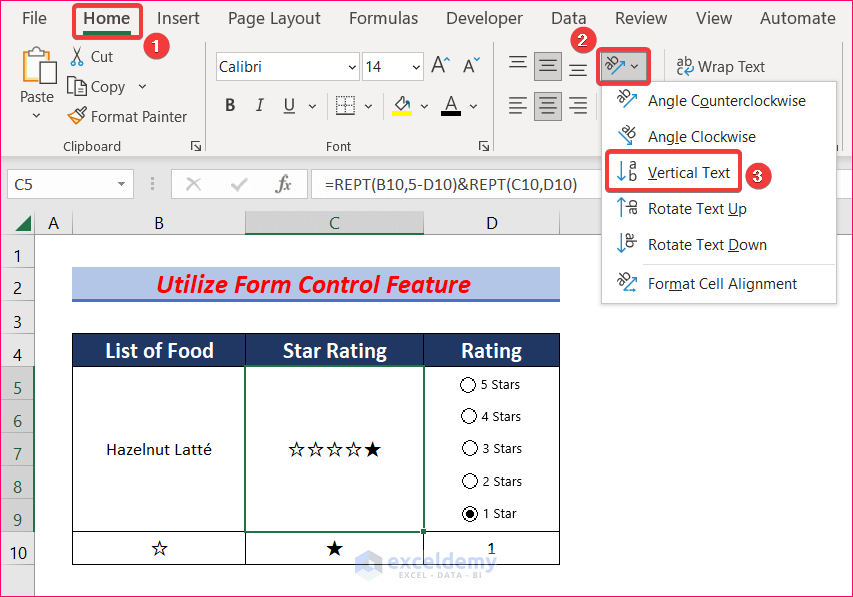
- As a result, the text will be vertically aligned now.
- Finally, change the font and color to improve its look.
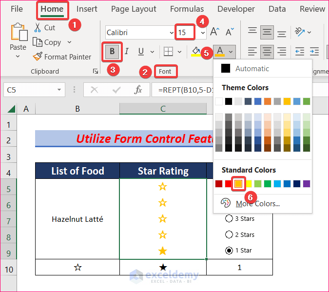
- Now if you click on different buttons, the Star Rating will be updated automatically.
Read More: How to Apply Alignment in Excel Conditional Formatting
4. Create Dropdown List to Create a Rating Scale
Steps:
- Create a column and write text ratings from Very Good to Very Poor in the column.

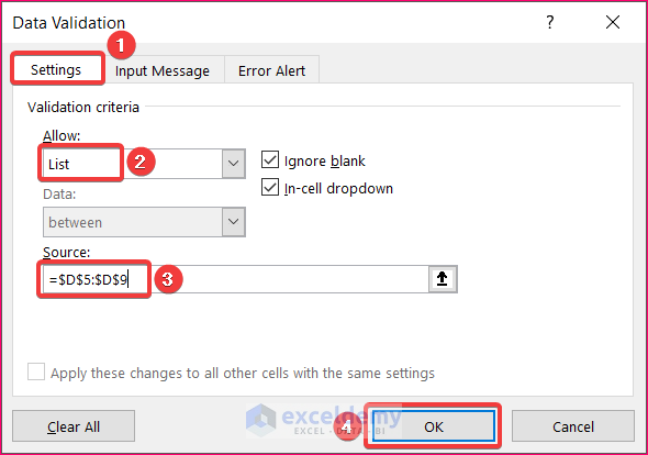
- Select the Rating column and, from the Data tab, go to Data Validation.
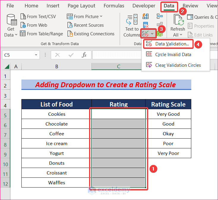
- The Data Validation dialogue box will appear. Go to the Settings tab and select List from Allow option.
- Choose the source as D5:D9 and click OK.
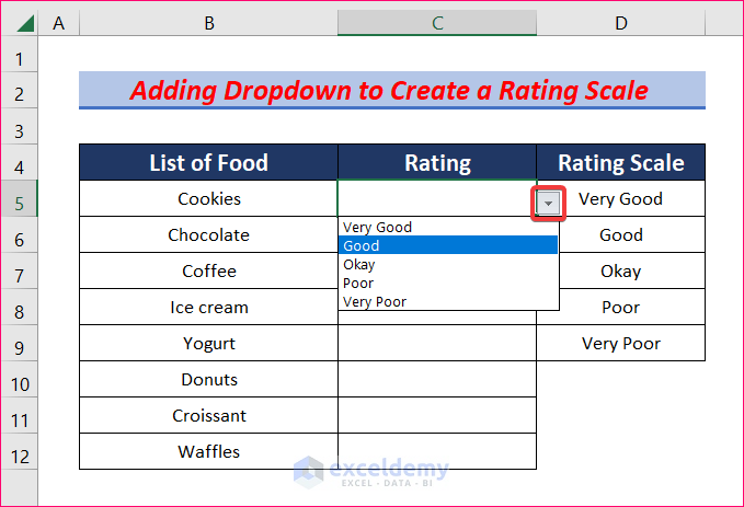
- Select any cell in column C and you will see a dropdown button beside it.
- Click on the dropdown button and you will have all the options to choose from.
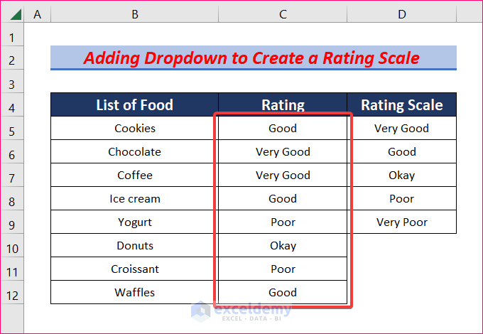
- Click on any of the options to rate the food item.
- You can rate all the food items on the list.
Notes
- You can follow the same steps to create rating scales with other symbols.
- Additionally, you can create 1-10 and 1-100 scales following the above procedures.
Download the Practice Workbook
Download this practice workbook to follow along while reading this article.
Related Articles
- How to Use Conditional Formatting on Text Box in Excel
- How to Copy Conditional Formatting to Another Cell in Excel
- How to Copy Conditional Formatting Color to Another Cell in Excel
- How to Copy Conditional Formatting to Another Sheet
- How to Copy Conditional Formatting to Another Workbook in Excel
- How to Copy Conditional Formatting with Relative Cell References in Excel
- How to Copy Conditional Formatting But Change Reference Cell in Excel
<< Go Back to Conditional Formatting | Learn Excel
Get FREE Advanced Excel Exercises with Solutions!
