[Solved]: Excel VLOOKUP Not Working with Numbers

The VLOOKUP function is a handy function to find things or values in a table or array. By utilizing the VLOOKUP function, we can get required column data in return from a specific table or array if the first column of the array meets certain criteria. However, we sometimes face errors when applying a criterion that consists of Numeric Data. In this article, I will show you how we can fix the issue when the VLOOKUP function is not working properly with numbers.

Excel VLOOKUP Not Working with Numbers: 2 Possible Solutions

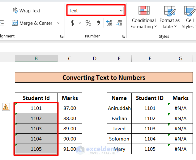
In this section, we will demonstrate 2 effective solutions to fix the stated problem in Excel with appropriate illustrations. But before jumping into the solutions, let’s see what our problem looks like. Here, I have attached a screenshot where I have two tables.

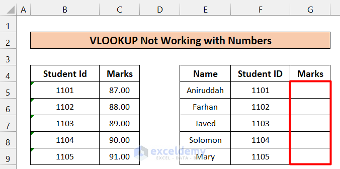
As we can see, on the left table, we have Some Student Ids and their Marks on a subject. On the right side, the table contains Names and Student IDs. Furthermore, the Marks column is supposed to be filled up using the VLOOKUP function from the left table. So we use the following formula to obtain Marks using the VLOOKUP function.

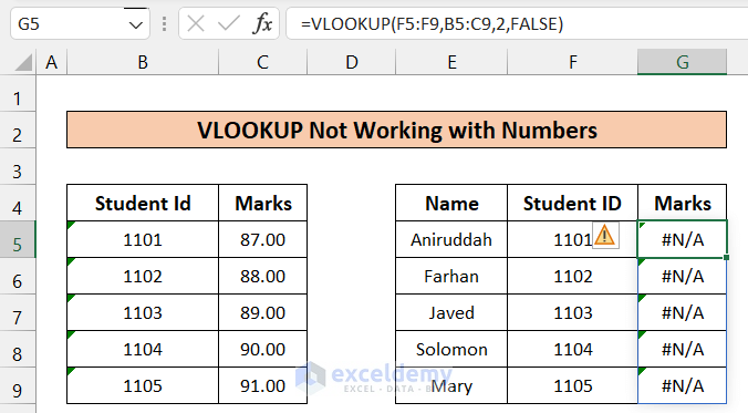
=VLOOKUP(F5:F9,B5:C9,2,FALSE)

Here we look for value form F5:F9(Student ID) in the 1st column of the B5:C9 array and return the 2nd column value(2) from the array which is Marks.

But, unfortunately, we got this error.

Now, to get rid of this error, we can follow either of the two solutions given below.

1. Converting Text to Numbers

It might be the case that the conditions that we have assigned to the VLOOKUP function are not uniformly formatted. For example, in this case, maybe the Student ID column on the two tables is not in a single format. To check and remove this error, follow the steps below.

Steps:

The easiest way to check is to pick any two corresponding cells from those two columns and write the following in any cell on the worksheet. (I have taken B5 and F5)

=F5=B5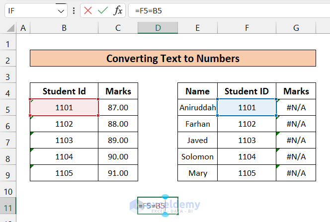

If the result comes TRUE, then they are in a uniform format. On the other hand, if the result comes FALSE, then they are not in a uniform format.

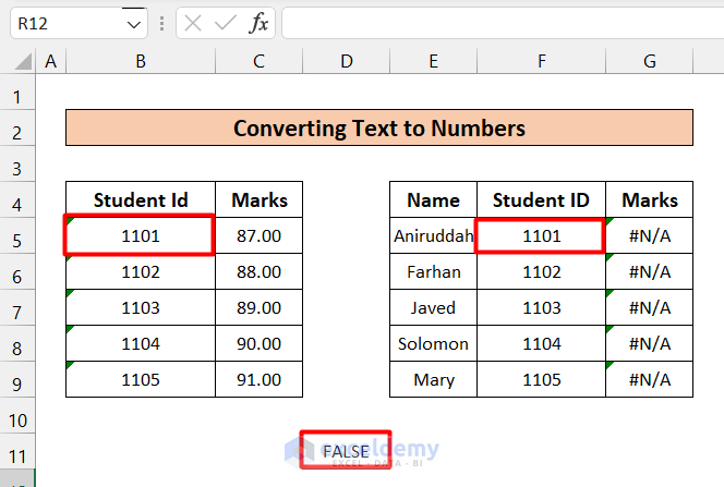
As the result is FALSE, hence the formatting needs to be changed to make those cells uniform. By inspecting, I found that the Student ID column of the left array is not in the Number format but rather in the Text option.

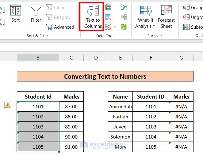
Now, to convert the column from text to numbers, first, select the column (B5:B9), and from the Data Tab, select the Text to Columns option.

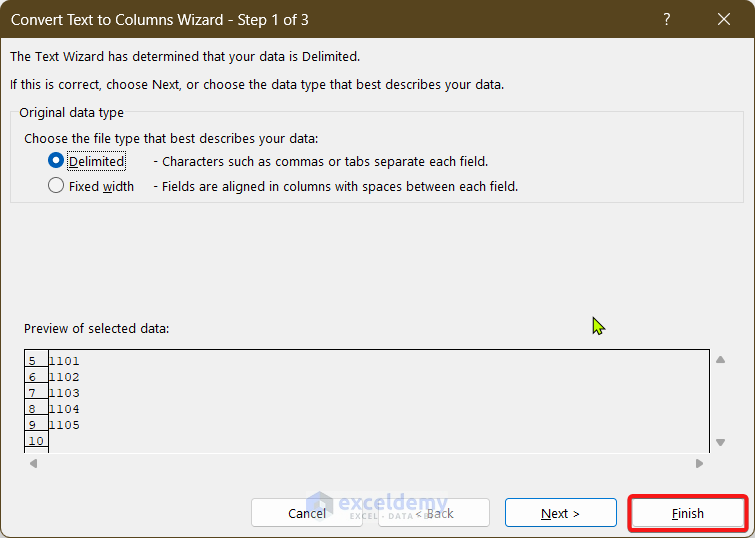
Now, a Convert Text to Columns Wizard dialogue box will appear like the figure below. From there, click on Finish.

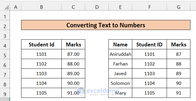
As a result, you will see that the previously shown error messages have gone.

2. Use of Ampersand Operator in the VLOOKUP formula

Now, for removing the error message, there is an alternative to change the formatting of the column data. Instead of changing the column format, we can slightly modify the VLOOKUP formula with an Ampersand sign (&) to gain our desired result without any error messages. To do this, follow the steps below.

Steps:

In the formula bar of G6 cell, write down the following formula.

=VLOOKUP(F5:F9&"",B5:C9,2,FALSE)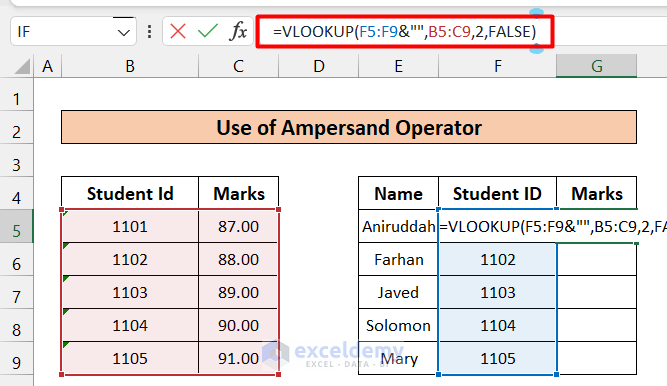

Here, we just added &“” after F5:F9. This will make the value received as Text. So we don’t need to manually change the formatting.
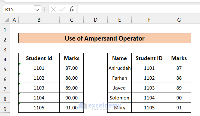
After pressing Enter, you will get the desired error-free result.

Fixing #VALUE! Error in VLOOKUP Formula

While using the VLOOKUP function, if the conditional cells contain more than 255 characters, then you will see the error like this below.

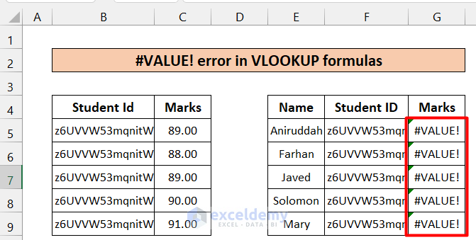
Here, in the Student Id column, the cell values are more than 255 characters, hence this error is showing. To solve the issue, instead of using the VLOOKUP function, use the combination of INDEX-MATCH functions. To learn more, follow the steps below.

Steps:

In cell G6, write down the following formula.

=INDEX($C$5:$C$9,MATCH(TRUE,INDEX($B$5:$B$9=$F5,0),0))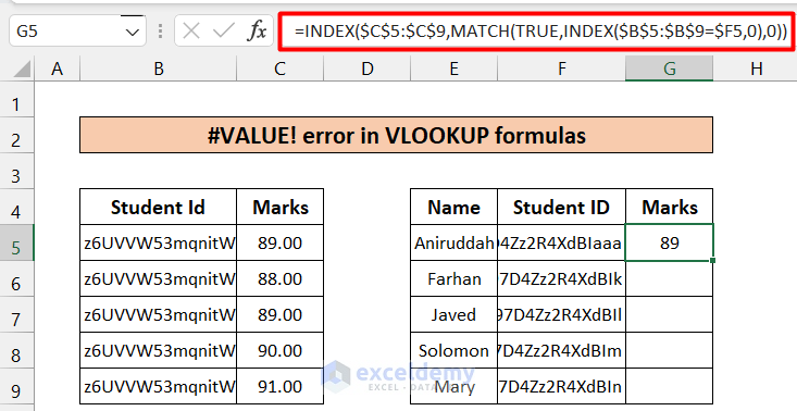

Now, autofill the rest of the cells with Fill Handle. You will get the desired result.

🎓How Does the Formula Work?

INDEX($B$5:$B$9=$F5,0)

It searches the value in of F5 in (B5:B9) column and returns an array of True(if matched) and False(If not matched).

MATCH(TRUE,INDEX($B$5:$B$9=$F5,0),0)

The MATCH function returns the row number which is TRUE in the array returned by the INDEX function

INDEX($C$5:$C$9,MATCH(TRUE,INDEX($B$5:$B$9=$F5,0),0))

This returns the value of the cell in the (C5:C9)array in which the row number is equal to the result of the MATCH function.

Things to Remember

Always check the data type of conditional cells before applying the VLOOKUP function

Download Practice Workbook

Download this practice workbook to exercise while you are reading this article.

VLOOKUP with Numbers Error.xlsx

Conclusion

That is the end of this article. If you find this article helpful in solving the issue when the VLOOKUP function not working with numbers then please share this with your friends. Moreover, do let us know if you have any further queries.