Creating a schedule is a part and parcel of many of our lives. Creating the schedule automatically will be immensely helpful for many people. If you are curious to know how you can create a schedule in Excel that updates automatically, then this article may come in handy for you. In this article, we will discuss how you can create a schedule in Excel that updates automatically.
How to Create a Schedule That Updates Automatically in Excel: Step-by-Step Procedure
Below we are going to present four step-by-step procedures following which you can create a dynamic schedule with a calendar. Which will update automatically as the date changes.
For better functionality, try to use the Microsoft 365 version for this method.
Step 1: Prepare Layout of Calendar
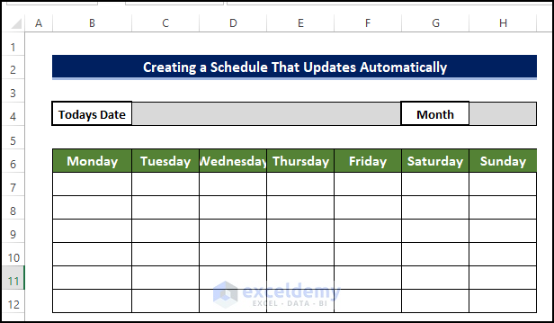
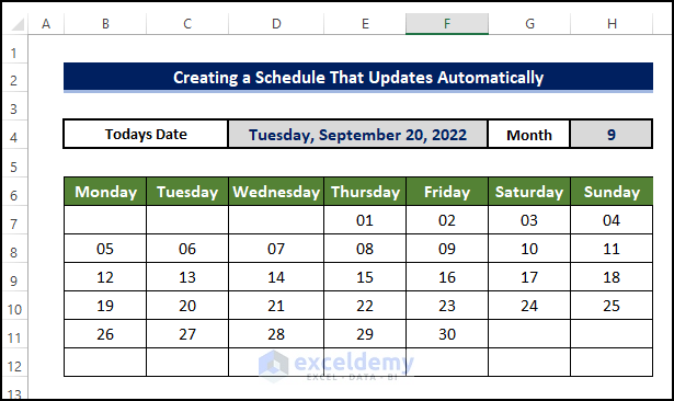
Before we delve into creating the schedule, it is imperative that we create the outline of our calendar first, in which we are going to implement the formulas.
Steps
- To begin, we need to prepare the layout of the outline of the calendar.
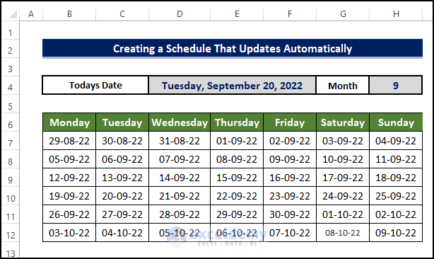
- To make it dynamic, we need to place the date and month on the sheet.
- The date and the month should be dynamic to today’s date.
- Our calendar will follow the weekdays starting from the Monday format.
Step 2: Formulize Calendar Outline
After we get the outline, it is time to formulate the calendar to make it dynamic. The functions like TODAY, MONTH, DATE, and WEEKDAY to achieve this.
Steps
- As we have the structure of the calendar plotted in the worksheet, we formulate the calendar to make it more dynamic.
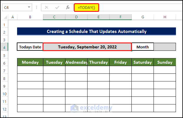
- To extract today’s date in the dataset, select cell D4, and enter the following formula:
=TODAY()
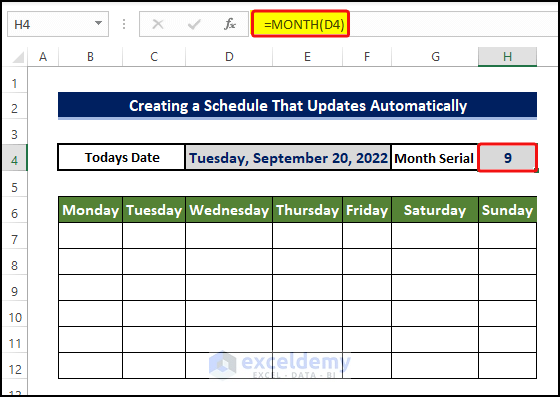
- Then select cell H4 and enter the following formula:
=MONTH(D4)
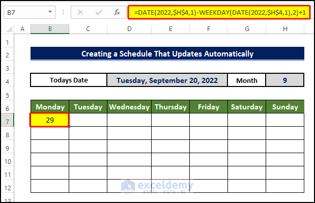
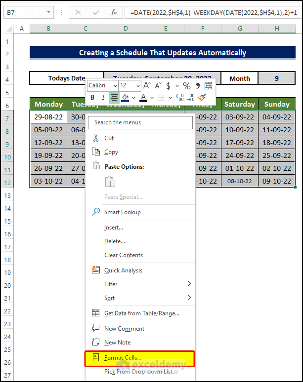
- Then select cell B7 and enter the following formula:
=DATE(2022,$I$4,1)-WEEKDAY(DATE(2022,$I$4,1),2)+1
Formula Breakdown
- DATE(2022,$I$4,1)
⮚ This will return the date in the proper date format. The month is from cell I4, and the year mentioned is 2022. And the date is 1.
- DATE(2022,$I$4,1)-WEEKDAY(DATE(2022,$I$4,1),2)+1
⮚ This will subtract the weekday from the date value. It will make sure that Monday stays at the front of the calendar.
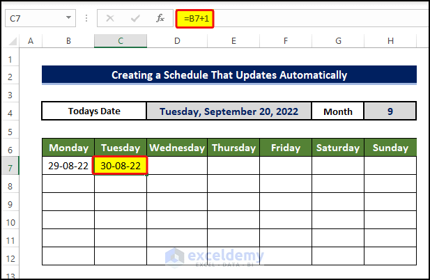
- Then select cell C7 and enter the following formula:
=B7+1
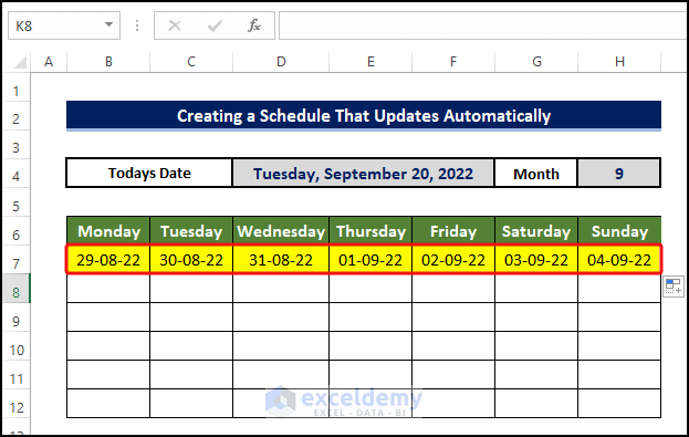
- Then drag the Fill Handle to the cell H7 from the cell B7.
- Doing this will fill the range of cells with dates starting from the 29th of October to the 4th of September.
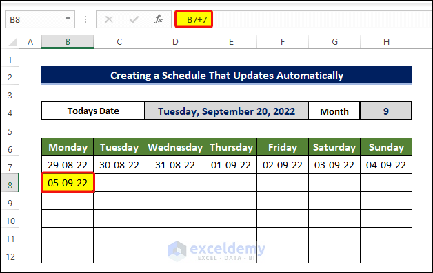
- Then again, select cell C8 and enter the following formula:
=B7+7
- And the Fill Handle to cell B12.
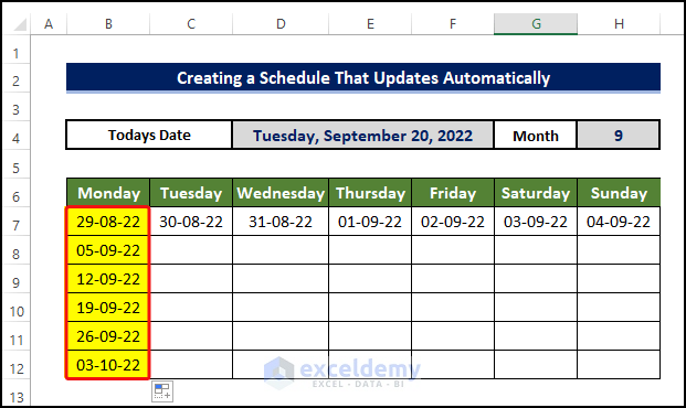
- Repeat the same process for the rest of the cells.
- Finally, we got the dates for all of the weekdays in a month.
- The right clicks on them and, from the context menu, click on Format Cells.
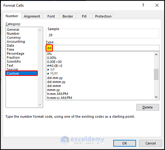
- In the Format Cells window, go to the Number tab.
- Then in the Custom options, select the Type field.
- In the Type field, enter dd only.
- This will allow the user to see only the day portion of the date.
- Click OK after this.
- After this, our calendar will now have the dates in a double-digit format.
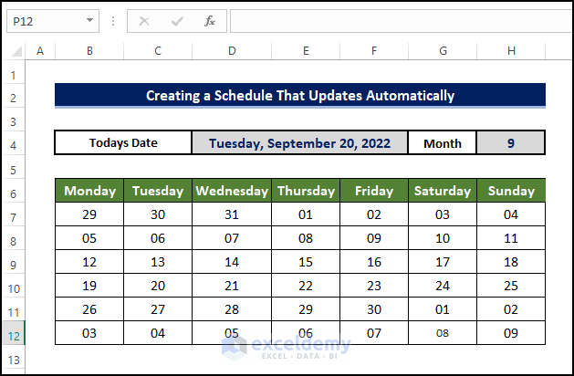
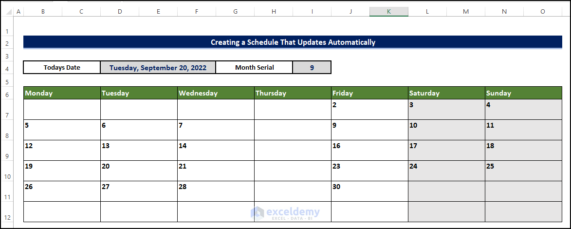
- We have the dates from the previous and next month.
- But we want to avoid that.
- To avoid that, we need to conditionally format the values.
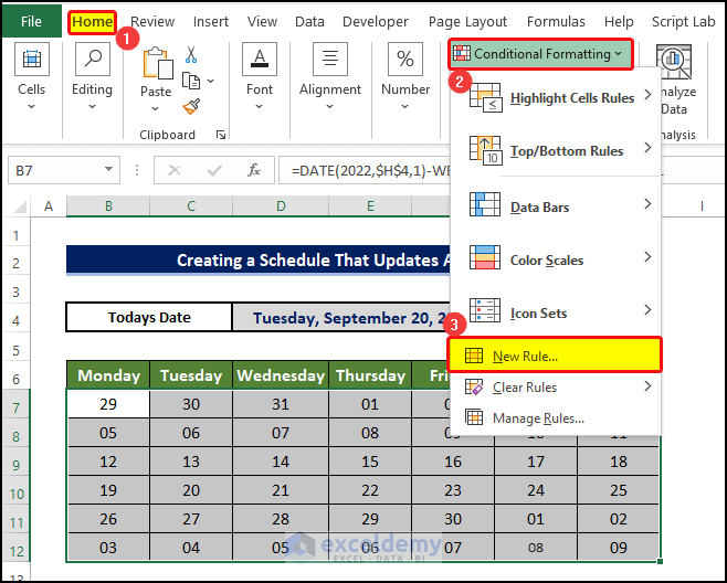
- For this, select the whole calendar and then go to the Home tab > Conditional Formatting > New Rule.
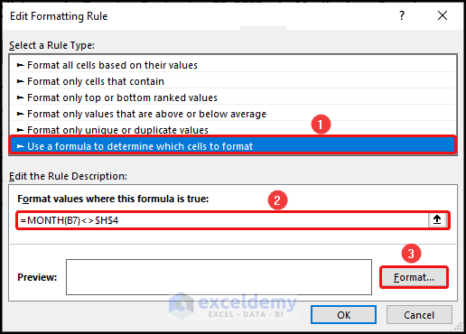
- In the Edit Formatting Rule window, select Use a Formula to Determine Which Cells to Format.
- Then enter the following formula:
=MONTH(B7)<>$H$4
- After entering the formula, click on the Format button.
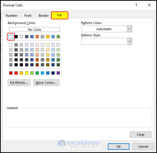
- In the Format Cells dialog box, click on the Fill tab.
- In the Fill tab, choose the color white as the fill color.
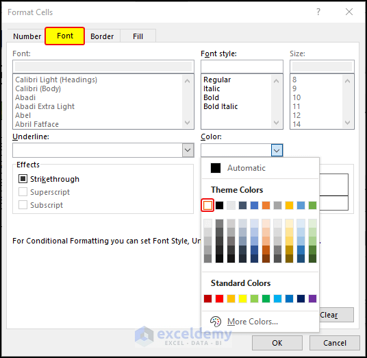
- Then switch to the Font tab, and choose the Color white as the font color.
- Click OK after this.
- The dates from the other months are now omitted from the view.
Step 3: Enlist All Scheduled Programs
We created the calendar and made it dynamic. Now we are going to fill out the monthly tasks or program schedules for each day. The date format should be maintained properly.
Steps
- The list of the programs in September month is enlisted with their scheduled date.
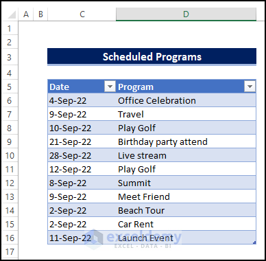
- And at the same time, we need to modify the existing table.
- We should add an extra cell just on the right side of each date.
- These cells will be used to store important event information.
Step 4: Link Programs with Calendar
We have both a calendar and a list of programs or events. We can now link the events with the calendar for each day. Functions like TEXTJOIN and FILTER are going to be used here.
Steps
- Now we are going to link the event list with the date in the calendar.
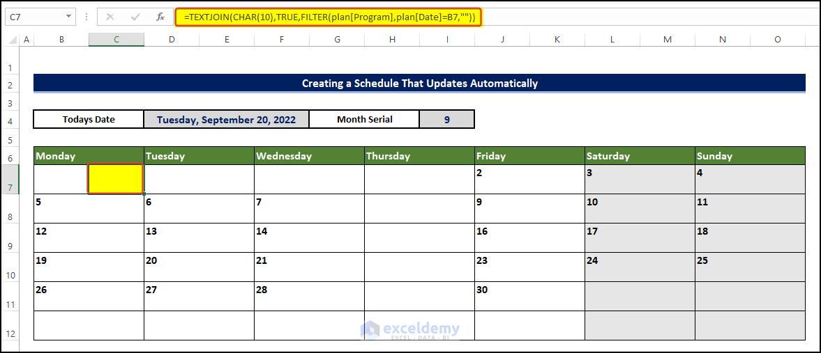
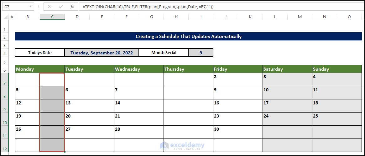
- To do this, select cell C7 and enter the following formula:
=TEXTJOIN(CHAR(10),TRUE,FILTER(plan[Program],plan[Date]=B7,""))
This formula will add the event associated with that date into the cell.
Formula Breakdown
- FILTER(plan[Program],plan[Date]=B7,””):
⮚ This formula will look for the value in cell B7 in the table plan’s program table header column. If the match is found, then it will present the whole row of information. Otherwise, it will extract a blank cell.
- TEXTJOIN(CHAR(10),TRUE,FILTER(plan[Program],plan[Date]=B7,””))
⮚Here, the TEXTJOIN function will join a separate line from the output of the FILTER function. The CHAR(10) [New line] here is acting as the delimiter between two or more text lines.
- Then drag the Fill Handle to cell C12.
- The cells are currently in a blank state because there is no event associated with the dates mentioned here.
- Repeat the same process for the subsequent cell.
- Select cell G7 and enter the following formula:
=TEXTJOIN(CHAR(10),TRUE,FILTER(plan[Program],plan[Date]=F7,""))
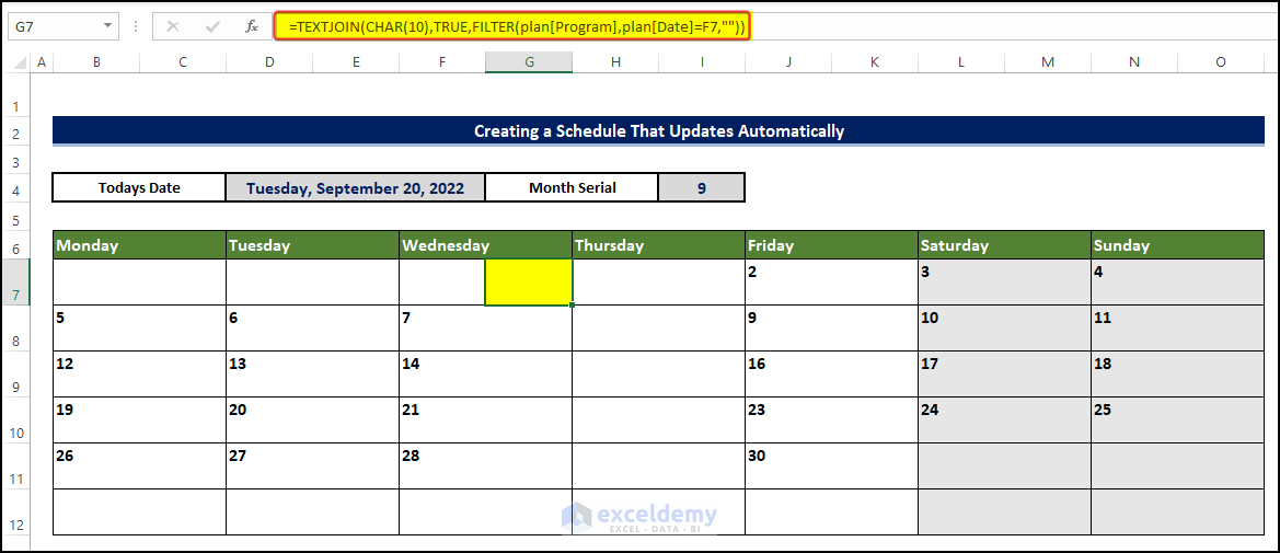
- And drag the Fill Handle to cell G12.
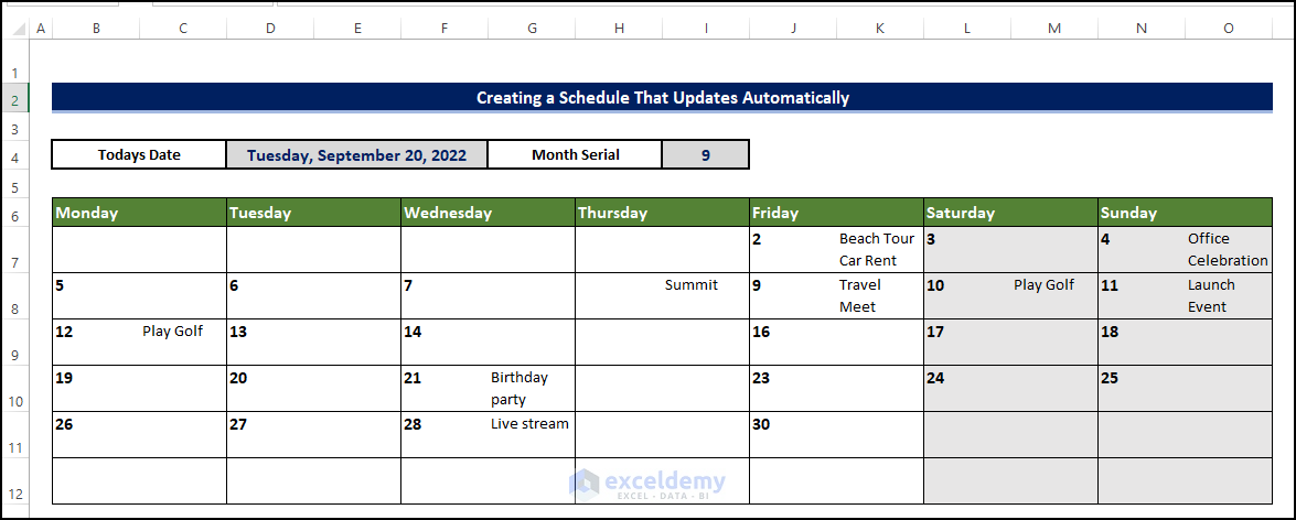
- Again, repeat the same process for the other weeks.
- By doing this, we will complete the calendar with the schedule.
Read More: How to Make a Daily Schedule in Excel
Download this practice workbook below.
Conclusion
To sum it up, the issue of how we can create a schedule in Excel that updates automatically by 4 different steps. For this problem, a workbook is available to download where you can practice these methods. Feel free to ask any questions or provide feedback through the comment section.
Related Articles
- How to Create a Weekly Schedule in Excel
- How to Create a Recurring Monthly Schedule in Excel
- How to Make an Hourly Schedule in Excel
<< Go Back to Make Schedule in Excel | Excel for Business | Learn Excel
Get FREE Advanced Excel Exercises with Solutions!

This was super helpful for what I was trying to do! Thank you so muchn
Hello, Andy W!
Thanks for your appreciation.
Regards
ExcelDemy
Hi,
I want to create a monthly excel attendance working schedule with formulate to calculate hours worked based on time in time out everyday for the whole month with daily hours totals excluding 1 hour lunch, total for the week and total for the month for each of the 10 employees. I have an example of one that was created with option of choosing time or off or on leave from the drop down arrow without typing. I like that but want to know how I can create mine from scratch.
Greetings,
I understand your query. You asked about attendence sheet for both monthly and weekly basis. But my suggestion will be to go on with the monthly basis assesment. In this way your job will be much smoother. Secondly I provided a demo sheet that actually contains the attendence with time picker drop down, and summation of total hour of work in a month.The time picker need to have a fixed time and they are specified below the sheet.You just need to enter the month and year in the beginning and then you can enter the in time and out time using the time picker.
The download file can be accessed from the link below,
https://www.exceldemy.com/wp-content/uploads/2023/04/Attendence-SheetMonthly.xlsx