To show negative numbers in Excel:
- Select the whole data range containing negative numbers.
- Click on the Home tab > Number group > Accounting Number Format icon.
Now you can see the negative numbers are inside the first bracket in the Accounting format.
Any number which is less than 0 (zero) is a negative number. Usually, this type of number refers to decreasing or lowering in quantity. We often use negative numbers to show a loss in business, penalty values, decrease in temperature, etc.
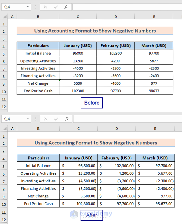
In this Excel tutorial, you will learn how to show negative numbers in Excel.
The following image illustrates the before-after scenario of showing negative numbers in Excel. Applying the Accounting format to the following dataset displays the negative numbers inside parenthesis.
5 Ways to Show Negative Numbers in Excel
You can use various predefined or custom number formats, Conditional Formatting, and VBA code to show negative numbers in Excel.
Here are 5 different methods to show negative numbers in Excel:
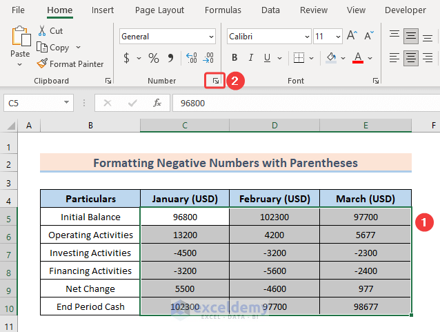
Using Parenthesis
There are some built-in formats in Excel to show negative numbers differently. One of them is showing them with parentheses. This option is available for cells that are Number or Currency formatted.
To show negative numbers with parenthesis, follow the steps below:
- Select the data range containing negative numbers.
- Click on the Number Format icon in the Number group.
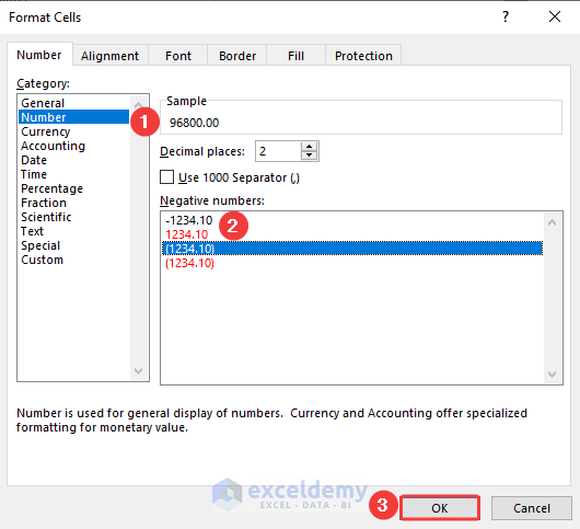
As a result, the Format Cells dialog box will appear. - In the Format Cells dialog box:
- Choose Number from Category.
- Select the option with parentheses.
- Click OK.
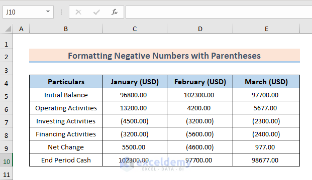
Now, look at the dataset. All the negative numbers are in parentheses.
Note: We can also avail of the Format Cells by using the keyboard shortcut Ctrl+1.
Read More: How to Add Negative Numbers in Excel
Using Custom Formatting
Using Custom formatting in Excel for showing negative numbers provides visual distinction by applying user specific styles, such as color variations, etc.
Let’s have a look at the procedure for applying Custom formatting to the negative numbers below:
- Select the cells containing negative numbers.
- Press Ctrl + 1 to open the Format Cells dialog box.
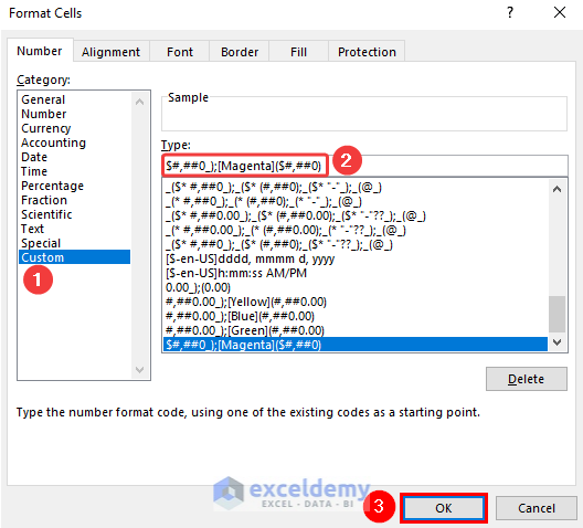
- Select Number tab > Category > Custom.
- Insert the target custom format in the Type box.
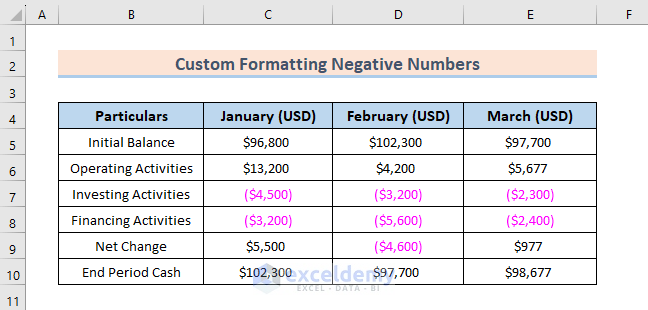
I entered $#,##0_);[Magenta]($#,##0) for showing the negative numbers in brackets and coloring them Magenta. - Click OK.
 All the negative numbers inside the dataset are in parentheses and colored in Magenta.
Note: In $#,##0_);[Magenta]($#,##0) custom format, the part before the semicolon in the code is to format the positive numbers, and the other one after the semicolon is to format the negative numbers. Excel offers 8 different color supports for user-defined number types. The names of these colors are: [Black], [White], [Red], [Green], [Yellow], [Magenta], [Cyan] and [Blue]. Color names need to be enclosed in brackets.
Read More: How to Put a Negative Number in Excel Formula
Using Accounting Formatting
Using the Accounting Number Format to display negative numbers provides a professional and standardized presentation of financial data.
To apply the accounting format, follow the steps below:
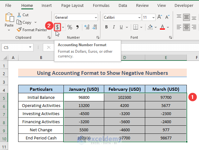
- Select the whole data range containing negative numbers.
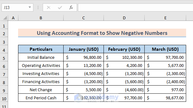
- Click on the Home tab > Number group > Accounting Number Format icon.
Now you can see the negative numbers are inside the first bracket in the Accounting format.
Read More: Excel Formula to Return Zero If Negative Value is Found
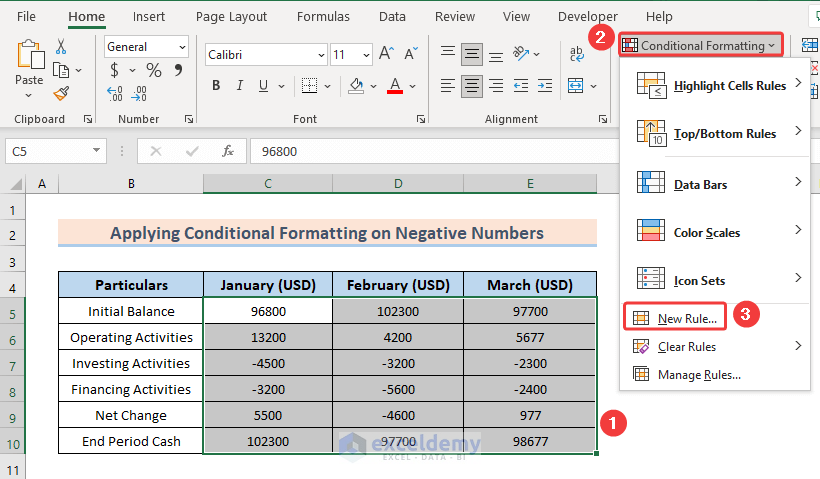
Applying Conditional Formatting
Conditional Formatting offers a variety of options to format cells in an Excel sheet based on conditions. When it comes to displaying negative numbers, conditional formatting can be particularly useful for improving the readability and visual impact of your data.
To differentiate the negative numbers by applying Conditional Formatting to them, follow the instructions below:
- Select the data range first.
- Next, select Home > Conditional Formatting > New Rule.
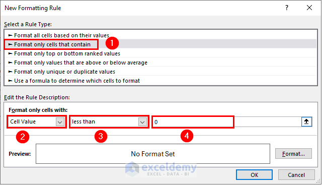
- In the New Formatting Rule dialog box, select the rule type Format only cells that contain.
- Edit the rule description as follows:
- For the 1st empty field, select Cell Value from the drop-down list.
- For the 2nd empty field, select less than from the drop-down list.
- For the 3rd empty field, put 0 in it.
- Click on the Format button to open the Format Cells dialog box.
- In the Format Cells dialog box:
- Go to the Font tab.
- Set a Font Style and Color of your choice.
Here, I have selected Italic font style and Red color. - Click OK inside the Format Cells dialog box.
- Click OK inside the New Formatting Rule dialog box.
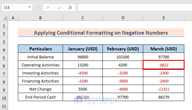
The negative numbers in the data range are shown with the Italic Font Style and Red color.
Here’s an image showing that if any of the numbers in the range are inserted as negative, it will be automatically formatted.
Using VBA
Excel VBA allows users to automate repetitive tasks, saving time and reducing errors by creating custom macros and scripts. VBA can facilitate the process of showing negative numbers in Excel by implementing user-defined rules for visual representation.
There could be 2 ways that you can use VBA to show negative numbers in Excel. They are:
Using VBA Subroutine
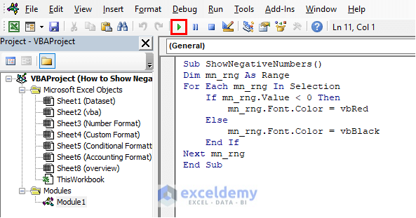
To distinguish the negative numbers using a VBA subroutine, follow the steps below:
- Open the VBA window by pressing Alt + F11 on your keyboard.
- Inside the VBA window, select Insert > Module.
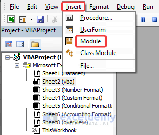
- Write the code below inside the Module.
Sub ShowNegativeNumbers() Dim mn_rng As Range For Each mn_rng In Selection If mn_rng.Value < 0 Then mn_rng.Font.Color = vbRed Else mn_rng.Font.Color = vbBlack End If Next mn_rng End Sub - Click on the Run Sub button.
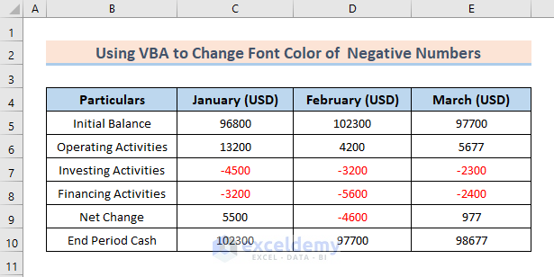
After running the Macro, you will see the negative numbers in the Red color font.
Assigning VBA Macro to a Button
You can also assign the VBA code to a button to operate this code conveniently.
Please follow the steps below to assign a code to a button:
- Select Developer tab > Insert.
- Choose Form Controls > Button.
- Drag a rectangle somewhere in the Excel sheet.
The Assign Macro window will pop up. - Select the Macro you want to run with this button and click OK.
- Give a name to this button.
In this case, the assigned name is Display Negative Numbers. - Select the data range with numbers (C5:E10).
- Click on the Button.
You will see the negative numbers in the Red color font.
What to Do When Negative Numbers Aren’t Showing with Parentheses in Excel
Although Excel can show negative numbers with brackets, it may occur to some users that the negative numbers cannot be shown with parentheses in Excel. The reason for that is the ($1,234.10) option isn’t available.
To solve this problem, follow the steps below:
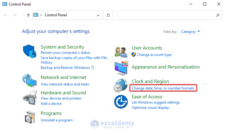
- Open the Control Panel.
- Choose the Change date, time, or number formats.
 The Region window will pop up.
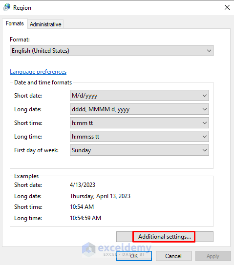
 - Inside the Region window, select Additional settings.
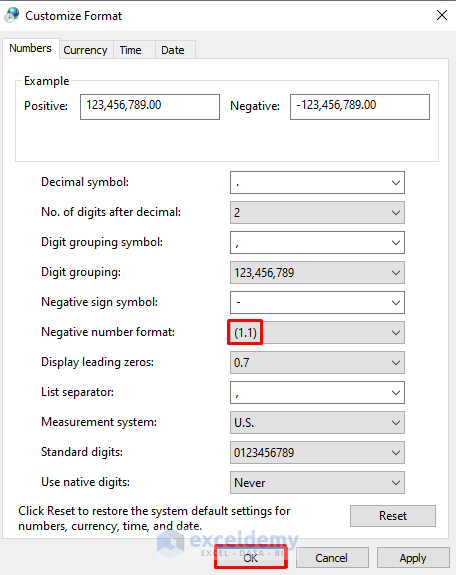
 A new window named Customized Format will pop out.
 - Inside the Customized Format window:
- Select the format (1.1) for the Negative number format.
- Click OK.
- Close the Excel file and reopen it.
Hopefully, this will solve your problem of negative numbers not showing in the Excel file.
Read More: How to Make a Group of Cells Negative in Excel
Download Practice Workbook
You can download the practice book from the button below.
Conclusion
To conclude, we used different number format features such as Accounting and Custom number format, Conditional Formatting, and VBA to display negative numbers in Excel. In terms of flexibility, using VBA codes could be your first choice. But if you are looking for simplicity, the Accounting format is there for you. If you have any questions or feedback regarding this article, please share them in the comment section.
Frequently Asked Questions
How do I auto-fill negative numbers in Excel?
To automatically fill negative numbers in Excel, follow these steps:
- Highlight the cells where you want to fill negative numbers.
- Start by typing a negative number in the active cell or entering it directly.
- Hover over the bottom right corner of the selected cell until a small square (the fill handle) appears.
- Click and drag the fill handle in the direction you want to fill the negative numbers. Excel will automatically fill the adjacent cells with increasing negative values.
How do I make Excel show negative times?
To display negative times in Excel, use the following steps:
- Input your time values in the desired cells, using the HH:MM:SS format.
- Select the cells containing time values, right-click, and choose “Format Cells.” Navigate to the “Custom” category.
- In the “Type” box, enter the custom time format as “[h]:mm:ss;[Red]-[h]:mm:ss” (without quotes). This format ensures negative times are displayed in red.
- Confirm the format by clicking OK.
How to make all negative numbers in a column positive in Excel?
You can use the ABS function to transform all negative numbers to positive ones in an Excel column. Inside the 1st cell of the column, put the formula =ABS(current cell address) and drag the fill handle up to the last cell of the column.
Related Articles
<< Go Back to Negative Numbers in Excel | Number Format | Learn Excel
Get FREE Advanced Excel Exercises with Solutions!
