How to Make Daily Sales Report in Excel (With Quick Steps)

If you are looking for some special tricks to make daily sales reports in Excel, you’ve come to the right place. In Microsoft Excel, there is one way to make a daily sales report. In this article, we’ll discuss every step of this method to make a daily sales report in Excel. Let’s follow the complete guide to learn all of this.

What Is Sales Report?

An organization’s sales report compiles, summarizes, and organizes information about its sales.

A sales report contains:

A record of each item’s sales against the target.
The number of engaged customers.
Continuation or discontinuation of existing customer records.
Comparing the new table with the old one is crucial.

How to Make Daily Sales Report in Excel (With Quick Steps)

In the following section, we will use one effective and tricky method to make daily sales reports in Excel. This section provides extensive details on every step of making daily sales reports in Excel. You should learn and apply to improve your thinking capability and Excel knowledge.

Step 1: Import Your Dataset

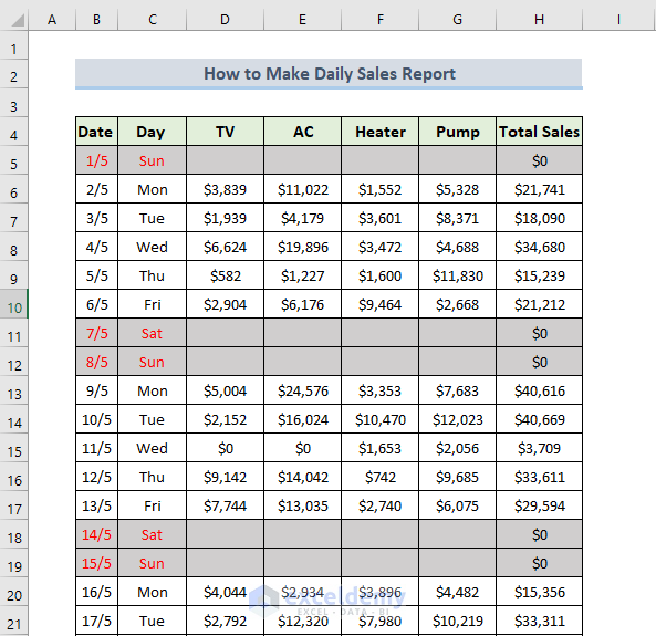
Here, we will demonstrate how to make daily sales reports in Excel. Let us first introduce you to our Excel dataset so that you are able to understand what we are trying to accomplish with this article. For creating a daily sales report, we have the following dataset of a companies’ s daily items price and total sales in May month. The everyday sales price of the TV, AC, Heater and Pump are shown in respective columns D, E, F, and G. Column H shows the total sales for each day, which we get by adding the columns D, E, F, and G. The following picture indicates the first 17 days sales data for May month of the company.

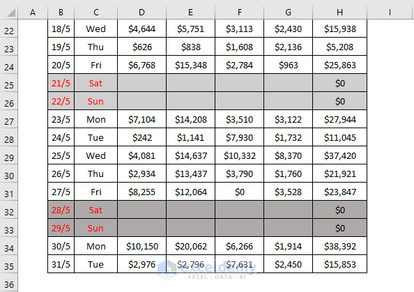
The following picture indicates the rest of the sales data for the May month of the company.

Step 2: Create Pivot Tables

Now, we are going to create a Pivot Table. To do this, we have to follow the following steps:

Firstly, select the range of cells B4:H35.
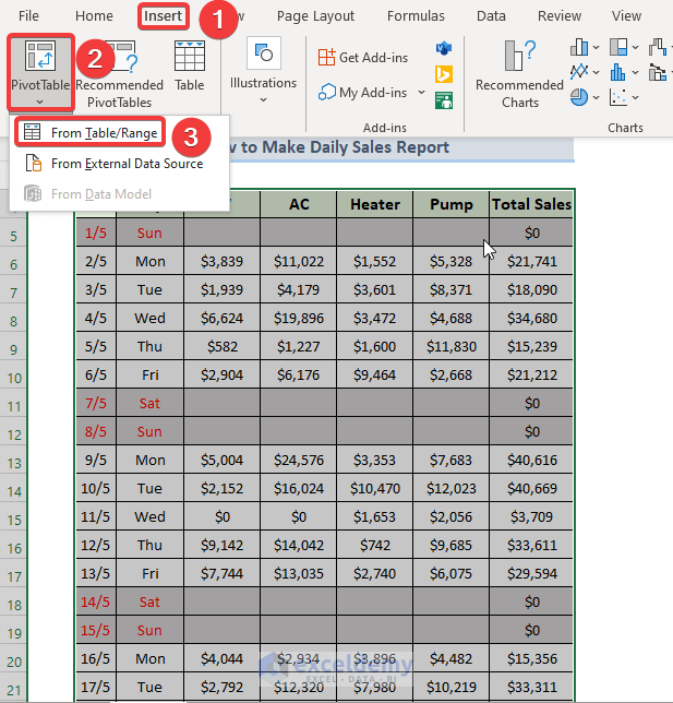
Next, select the Insert tab. Then, select PivotTable > From Table/Range.

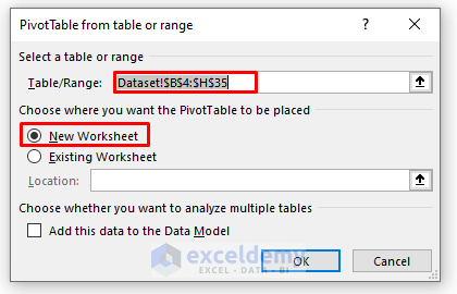
When the PivotTable from table or range dialog box appears, choose New Worksheet. Then, click on OK.

As a consequence, there will be a new worksheet. Your Pivot Table Fields will appear on the right.
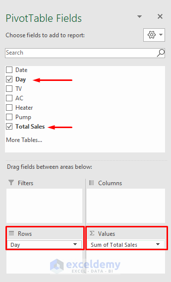
After that, check Day and Total Sales.
Then, place Day in Rows, and Total Sales in the Values section.

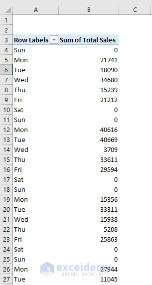
As a result, you will be able to create a pivot table containing the day and total sales of the dataset like the following.

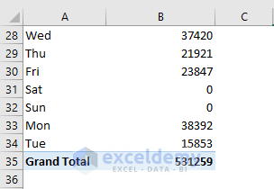
The rest of the data in the pivot table are the following.

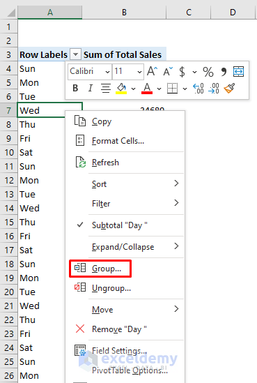
If we want to create a pivot table containing each week’s total sales you need to right-click on the previous table and select Group.

Next, check the Starting at. Select Days. Then, enter 7 in the Number of days box.

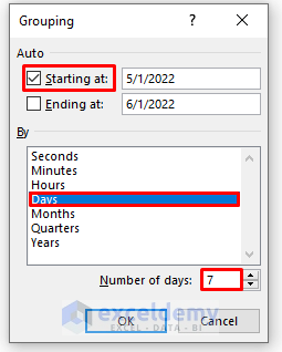
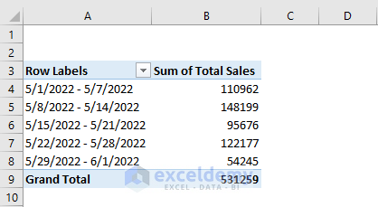
As a consequence, you will be able to create a pivot table containing each week’s total sales, like the following.

Step 3: Inset Slicer

Now, we will insert a slicer into our spreadsheet. It gives us a lot of flexibility while filtering our data. To do this, you have to follow the following steps.

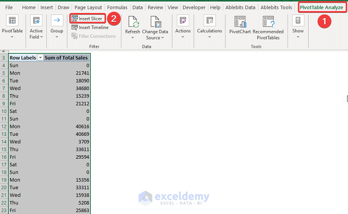
Firstly, select the whole pivot table.
Go to Pivot Table Analyze and select Insert Slicer.

Then, select Day in the Insert Slicers dialog box.

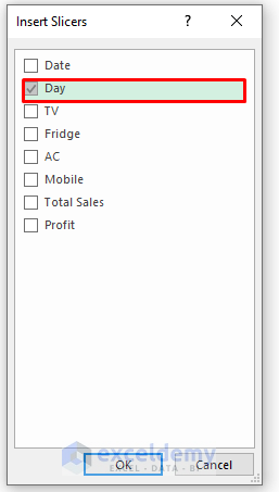
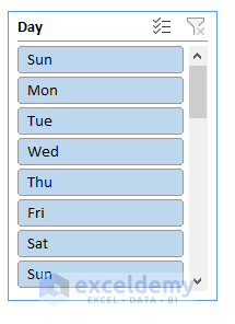
As a consequence, you will be able to create a slicer like the following.

Step 4: Insert Charts for Pivot Tables

Now, we are going to create four different charts for the daily sales reports. To do this, we have to follow the following steps.

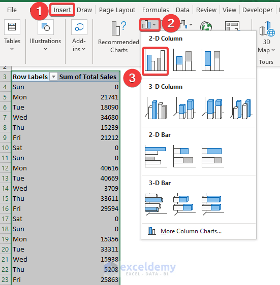
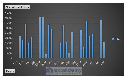
To create a chart, select the range of data and go to the Insert tab. Next, select the 2-D Column chart.

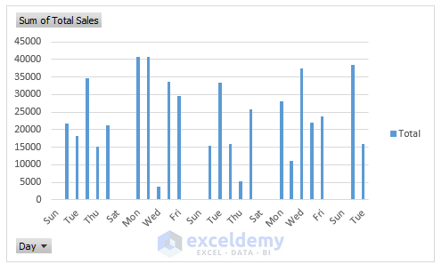
As a consequence, you will get the following chart.

To modify the chart style, select Design and then, select your desired Style 4 option from the Chart Styles group.

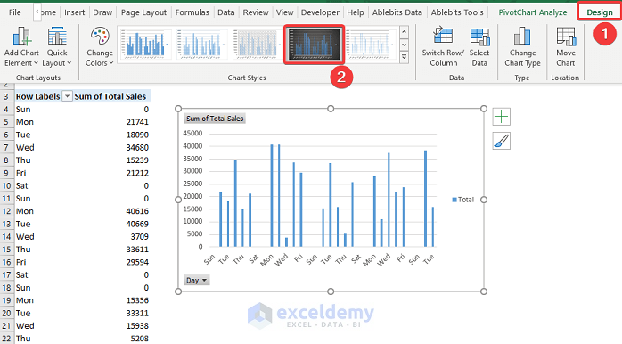
As a consequence, you will get the following modified chart.

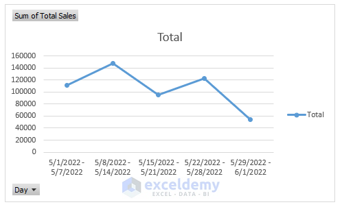
To create another chart, select the range of data and go to the Insert tab. Next, select the 2-D Line chart.

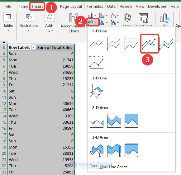
As a consequence, you will get the following chart.

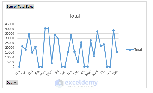
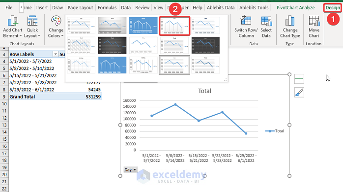
To modify the chart style, select Design and then, select your desired Style 6 option from the Chart Styles group.

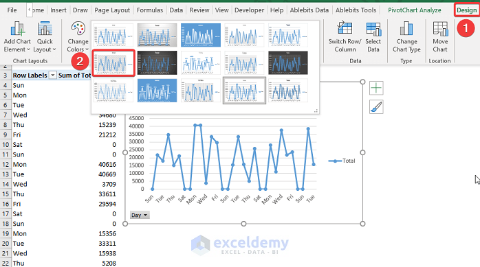
As a consequence, you will get the following modified chart.

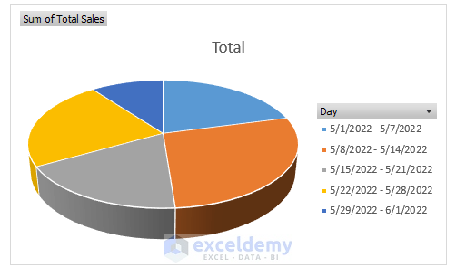
To create a Pie chart, select the range of data and go to the Insert tab. Next, select the 3-D Pie chart.

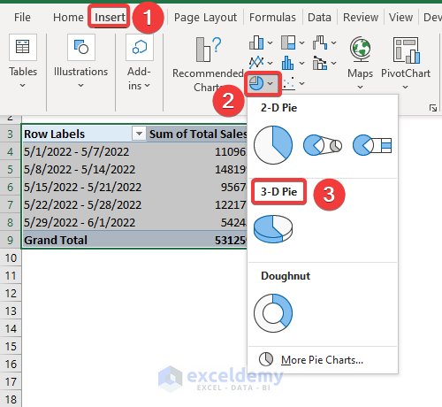
As a consequence, you will get the following Pie chart.

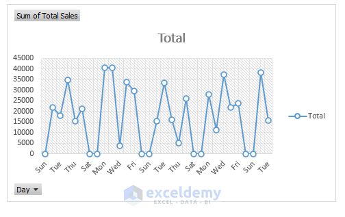
To create another chart, select the range of data and go to the Insert tab. Next, select the 2-D Line chart.

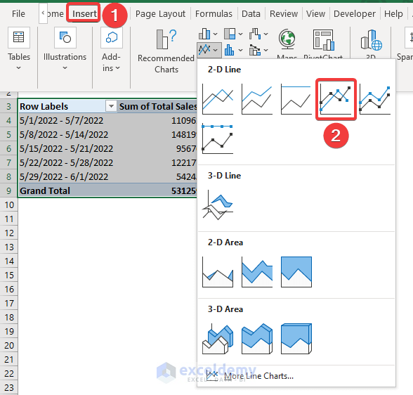
As a consequence, you will get the following chart.

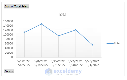
To modify the chart style, select Design and then, select your desired Style 4 option from the Chart Styles group.

As a consequence, you will get the following modified chart.

Step 5: Generate Final Report

Now, we will create final reports. To do this, we are going to show our charts in a new sheet as a Report.

To create a report, at first, you have to create a new sheet and set the name of that sheet as Report.
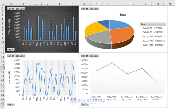
Next, you have to copy every chart by pressing ‘Ctrl+C’ and go to the Report sheet, and press ‘Crl+V’ to paste it.
As a consequence, you will get the Daily Sales report like the following.

Download Practice Workbook

Download this practice workbook to exercise while you are reading this article.

Daily Sales Report.xlsx

Conclusion

That’s the end of today’s session. I strongly believe that from now on you may be able to make daily sales reports in Excel. If you have any questions or recommendations, please share them in the comments section below.