How to Add a Blank Option to Drop-Down Lists and Create Drop-Down List Without a Blank Options

ADD:

Method 1 – Use an Empty Cell as Reference to Add a Blank Option in a Drop-Down List

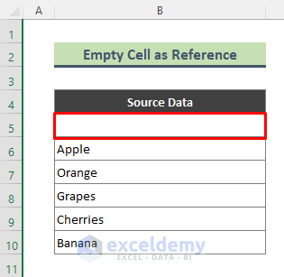
Insert a Blank Cell:
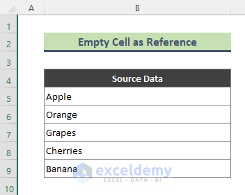
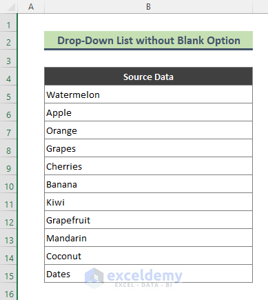
- Begin by adding an empty cell at the beginning of your source list. For example, let’s say you have a dataset containing various fruit names, and you want to create a drop-down list based on this data.

- Make sure that Cell B5 (or any other empty cell) is left blank.

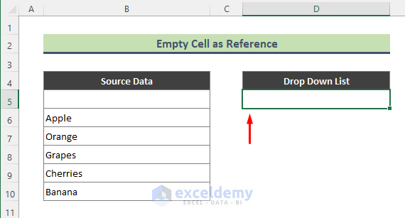
Create the Drop-Down List:
- Position your cursor in Cell D5 (or any other desired cell where you want the drop-down list).

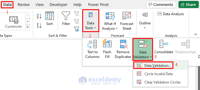
- Navigate to the Excel Ribbon and go to Data > Data Tools > Data Validation > Data Validation.

- The Data Validation dialog will appear.
Configure the Settings:
- In the Settings tab, select List from the Allow section.
- Specify the source list (which includes the fruit names along with the blank cell).
- Make sure to uncheck the Ignore Blank option.
- Click OK to create the drop-down list.

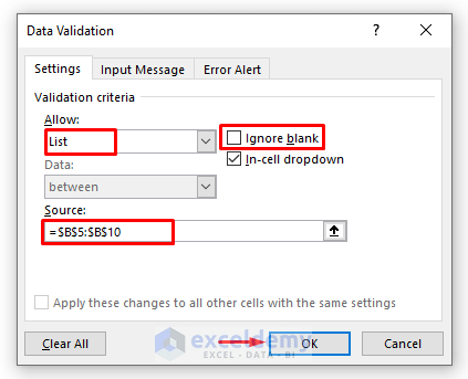
As a result, you’ll have a drop-down list that includes the blank option.

Method 2 – Manually Type List Values to Add a Blank Option in a Drop-Down List

Position the Cursor:
- Place your cursor where you want to create the drop-down list.
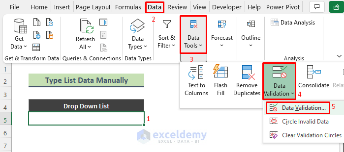
Access Data Validation:
- Navigate to Data > Data Tools > Data Validation > Data Validation. This will open the Data Validation dialog.
- While creating a drop-down list, you can enter source data manually in the Data Validation dialog. To perform the task, follow the below steps.

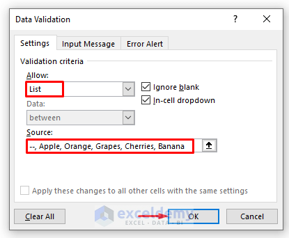
Configure the Settings:
- In the Settings tab, select List from the Allow field.
- In the Source field, type a double dash (- -) at the beginning of each item you want to display in the drop-down list.
- Click OK to confirm.

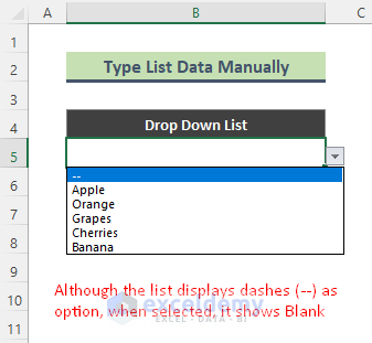
As a result, you’ll have a drop-down list that includes the double dash (- -) as an option. However, when you select it, the cell will display a blank value.

CREATE:

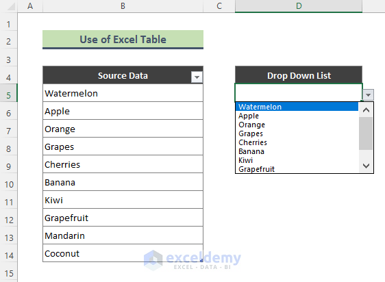
Method 1: Using an Excel Table to Create a Drop-Down List without Blank Options

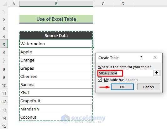
Convert the Source Data to an Excel Table:
- Before creating the drop-down list, convert your original source data range into an Excel table. This step is essential because it ensures that your drop-down list remains dynamic even if you add or remove items from the source table.

- To create an Excel table, select the data range (e.g., the list of fruits) and press Ctrl + T.

- Let’s convert the original data range to an excel table using Ctrl + T.

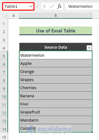
- Next, use the Name Box (located near the formula bar) to name the table. For example, you can name it Table1.

Create the Drop-Down List:
- Choose the cell where you want to place the drop-down list (e.g., Cell D5).
- Go to the Data tab and click on Data Validation.
- In the Data Validation dialog, select List under the Allow section.
- In the Source field, enter the formula =$Table1. Note that you should include the dollar sign ($) before the cell reference of the source data.
- Click OK to create the drop-down list.

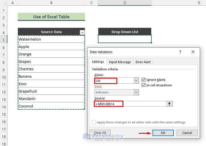
As a result, you’ll have a drop-down list without any blank options.

If you later add new items to the source table, the drop-down list will automatically update accordingly.

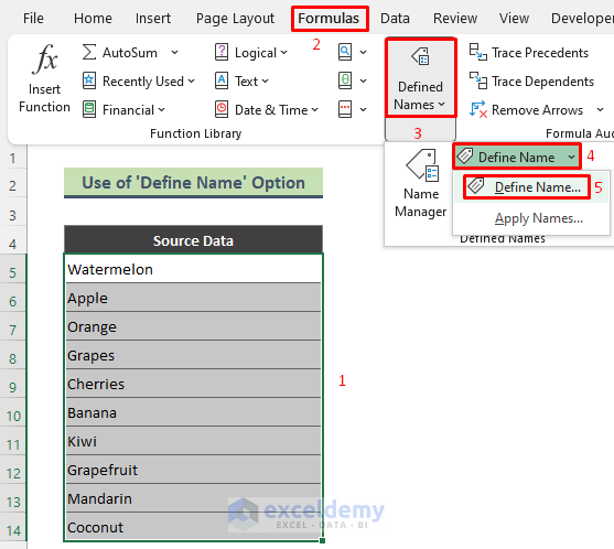
Method 2 – Using a Named Range to Create a Drop-Down List without Blank Options

Define a Named Range:
- Begin by selecting the entire data range (B5:B14) that you want to use for your drop-down list.
- Go to Formulas > Defined Names > Define Name > Define Name.

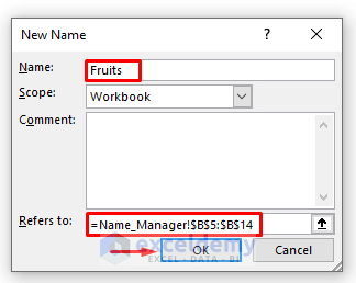
- In the New Name window, enter a descriptive name (e.g., “Fruits”) in the Name field.
- Check the Refers to box and press OK to complete the naming process.

Create the Drop-Down List:
- Choose the cell where you want to place the drop-down list (e.g., Cell D5).
- Go to the Data tab and click on Data Validation.
- In the Data Validation dialog, select List under the Allow section.
- In the Source field, enter =Fruits (the name you defined earlier) and press OK.

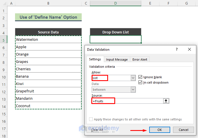
As a result, we will create the below drop-down list without a blank option.

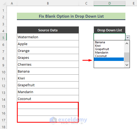
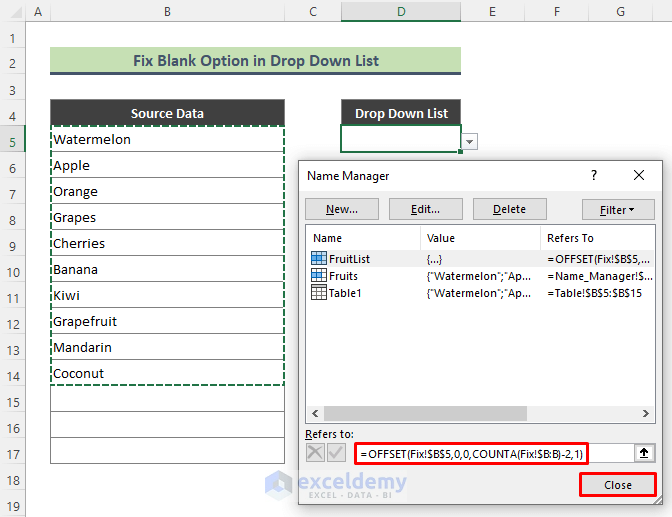
Removing Blank Options:
- Suppose you already have a drop-down list (created from a named range called “FruitList”) that includes blank options.

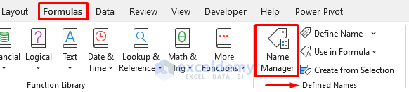
- Go to Formulas > Name Manager (from the Defined Names group).

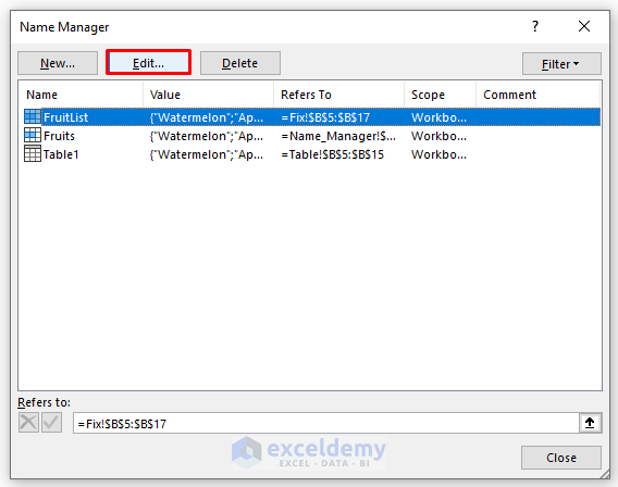
- In the Name Manager dialog, select your range (e.g., “FruitList”) and click Edit.

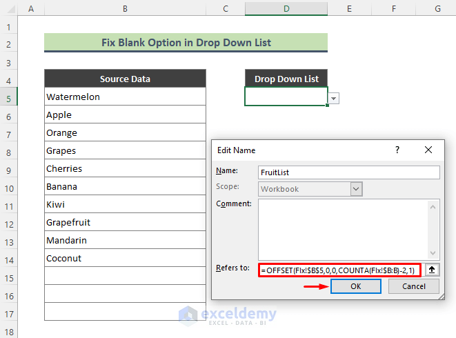
- In the Edit Name dialog, enter the following formula in the Refers to field:

=OFFSET(FIx!$B$5,0,0,COUNTA(FIx!$B:B)-2,1)

- Press OK to confirm.

Result:

The drop-down list will now display all the fruits from the named range, excluding any blank options.

How Does the Formula Work?

COUNTA(FIx!$B:B)-2

- The COUNTA function counts the number of non-empty cells in column B of the sheet named “FIx.”
- In this case, it returns a value of 10 because there are 10 non-empty cells in that column.
- We subtract 2 from this count because there are two cells in the range that are not fruits (presumably headers or other non-fruit data).

OFFSET(FIx!$B$5,0,0,COUNTA(FIx!$B:B)-2,1)

- The OFFSET function returns a reference to a range based on a given reference cell (in this case, Cell B5 on the “FIx” sheet).
- The parameters are as follows:
- Starting reference: Cell B5
- Rows offset: 0 (no vertical offset)
- Columns offset: 0 (no horizontal offset)
- Height: COUNTA(FIx!$B:B) – 2 rows (excluding the non-fruit cells)
- Width: 1 column (since we want a single-column range)
The resulting range includes the fruit names without any blank options.