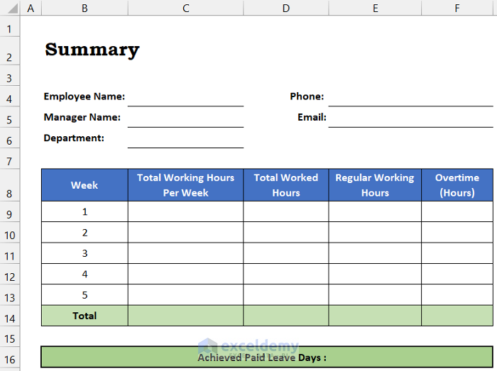
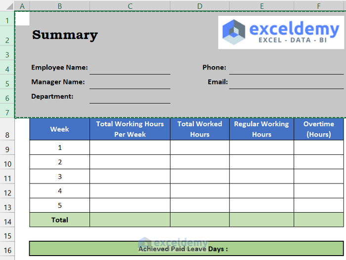
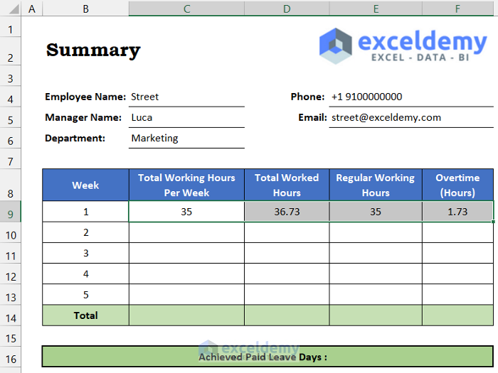
Step 1: Design Primary Summary Layout
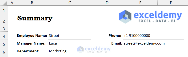
- Select cell B2 and enter the title of this sheet Summary.
- Rename the sheet name in the Sheet Name Bar as Summary to easily find the sheet.
- In the range of cells B4:B6 and D4:D5, enter the following entities:
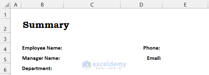
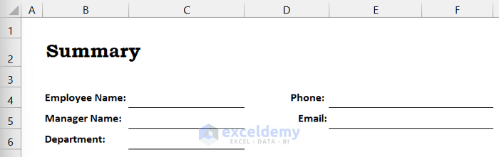
- Format the neighboring cells of those mentioned cells to ensure the input location of those data.
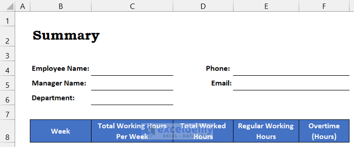
- In the range of cells B8:F8, enter the following table headings:
- Denote in range of cells B9:B13, 1-5 for five weeks of that month.
- Name cell B14 as Total to show the total of all the columns.
- Name cell D16 as Achieved Paid Leave Days.
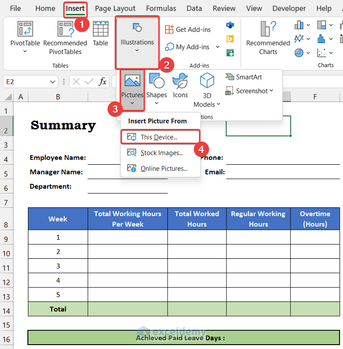
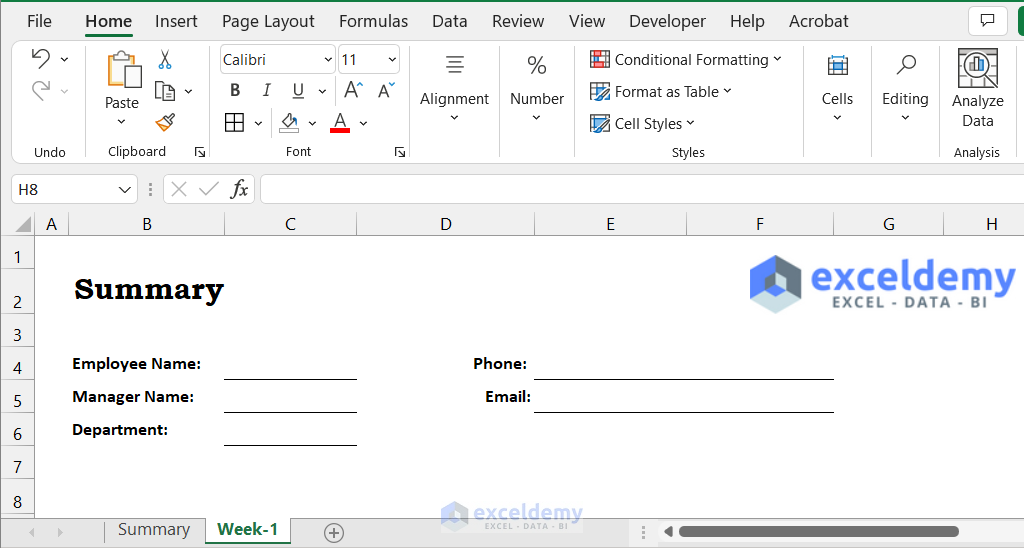
- Insert your company logo.
- Select cell E2.
- In the Insert tab, click on the drop-down arrow of the Illustration > Picture option.
- Choose the This Device option.
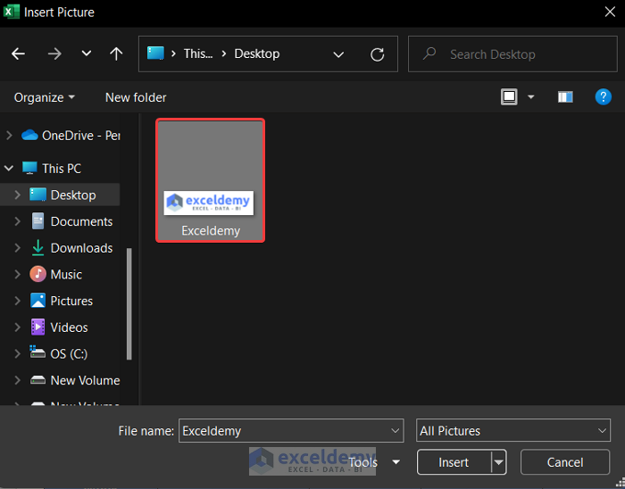
- As a result, the Insert Picture dialog box will appear.
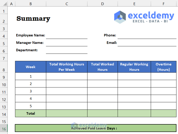
- Choose your institution’s logo and click Insert. In our case, we insert our website’s logo.
Our preliminary summary design is completed.
Step 2: Create a Comp Time Tracker Table
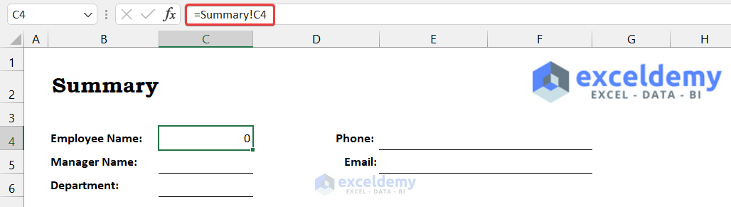
- Create a new sheet and rename it Week 1.
- Select the entire row 1:7 in the Summary sheet and press ‘Ctrl+C’ to copy everything.
- Go to the Week 1 sheet and press ‘Ctrl+V’ to paste.
- In cell C5, enter the following formula to extract the value of the employee’s name from the Summary sheet.
=Summary!C4
- Press Enter.
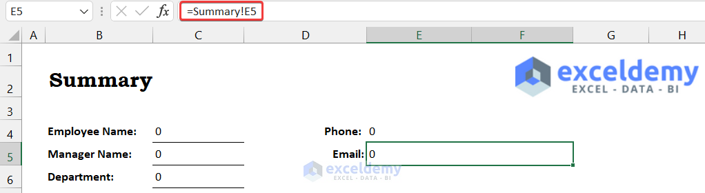
- Enter the following types of formulas in the range of cells C5:C6 and E4:E5.
- Press Enter to store the formula in that cell.
- We want to add a weekly summary report to this sheet.
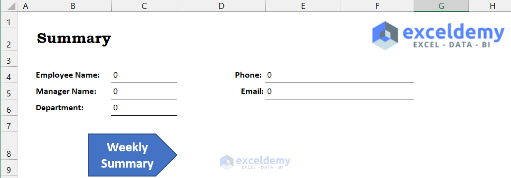
- In the Insert tab, click the drop-down arrow of the Illustration > Shapes option. Choose a shape according to your desire. In our case, we choose the Arrow: Pentagon shape.
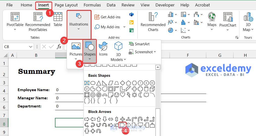
- Enter the title Weekly Summary inside the shape.
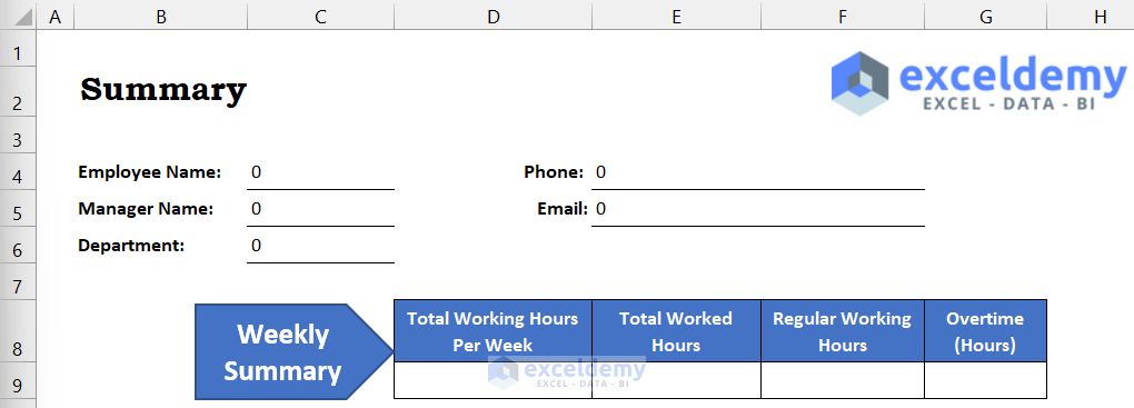
- In the range of cells D8:G8, write down the following summary table headings.
- Allocate a cell below every heading to show their results.
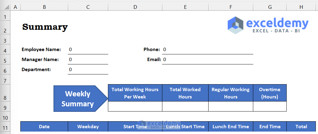
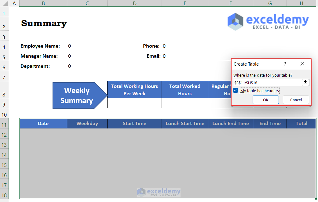
- In the range of cells B11:H11, enter the following table headings to create the comp time tracker.
- Select the range of cell B11:H18 and press ‘Ctrl+T’ to convert the dataset into a table.
- A small window called Create Table will appear.
- Check the option My table has headers and click OK.
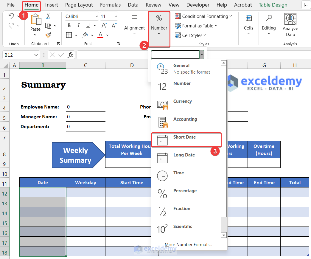
- Modify the cell format. Select the range of cells B12:B18, and choose the Short Date format from the Number group.
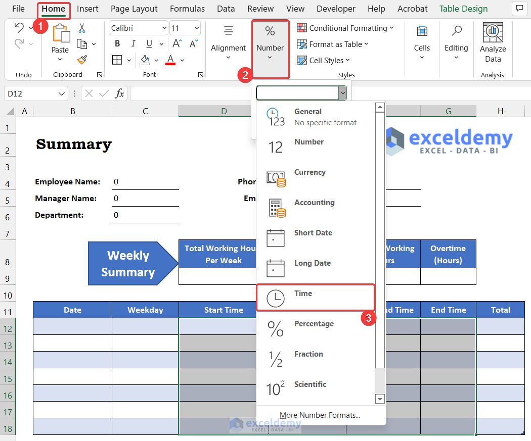
- For the range of cells D12:G18, modify the cell format from General to Time.
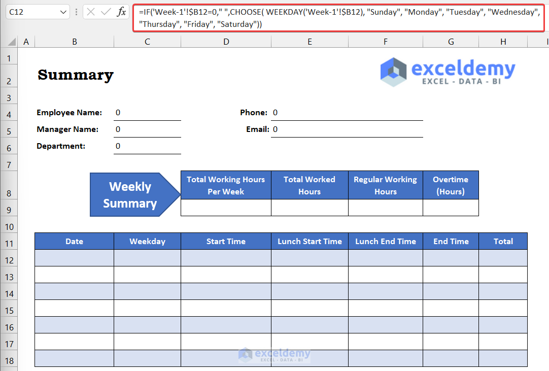
- Enter the following formula in cell C12 to get the weekday’s name. For that, we will use the IF, CHOOSE, and WEEKDAY functions:
=IF([@Date]=0," ",CHOOSE( WEEKDAY([@Date]), "Sunday", "Monday", "Tuesday", "Wednesday", "Thursday", "Friday", "Saturday"))
- Press Enter.
- To get the total working hours, enter the following formula into cell H12 using IFERROR, IF, COUNT, AND, and LEN functions.
=IFERROR(IF(COUNT(Comp_Time[@[Start Time]:[End Time]])=4,(IF([@[End Time]]<[@[Start Time]],1,0)+[@[End Time]])-[@[Lunch End Time]]+[@[Lunch Start Time]]-[@[Start Time]],IF(AND(LEN([@[Start Time]])<>0,LEN([@[End Time]])<>0),(IF([@[End Time]]<[@[Start Time]],1,0)+[@[End Time]])-[@[Start Time]],0))*24,0)
- Press Enter.
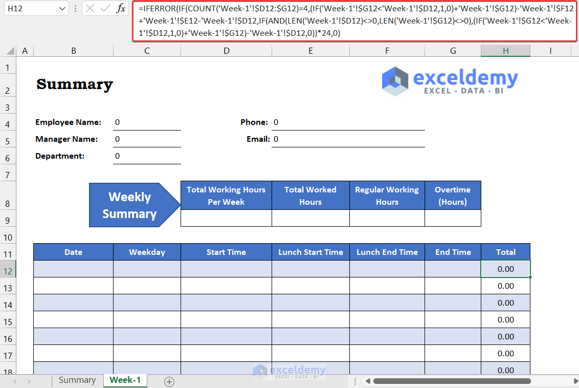
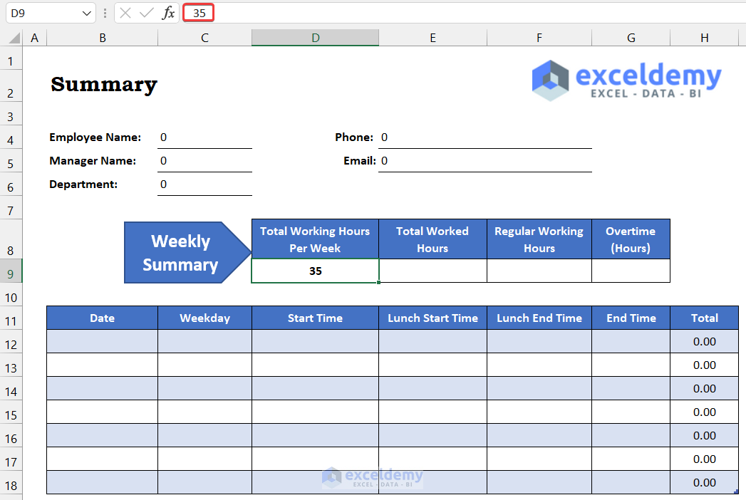
Our weekly tracker is ready. Now, we are going to complete the week’s summary table.
- In cell D9, enter the total working hours per your organization’s policy. We entered 35 hours as our policy.
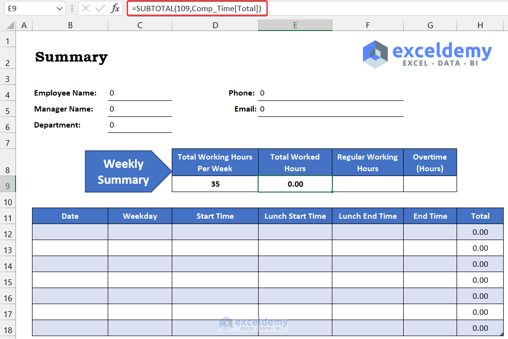
- In cell E9, enter the following formula to get the total worked hours using the SUBTOTAL function.
=SUBTOTAL(109,Comp_Time[Total])
- Press Enter.
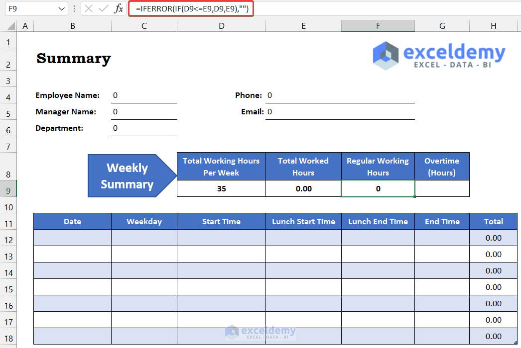
- To get the value of regular working hours, enter the following formula in cell F9:
=IFERROR(IF(D9<=E9,D9,E9),"")
- Press Enter.
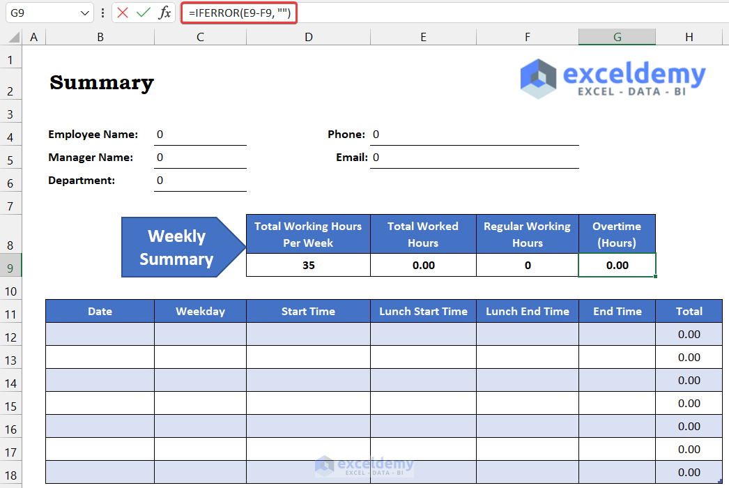
- To get the overtime value, enter the following formula in cell G9:
=IFERROR(E9-F9, "")
- Press Enter.
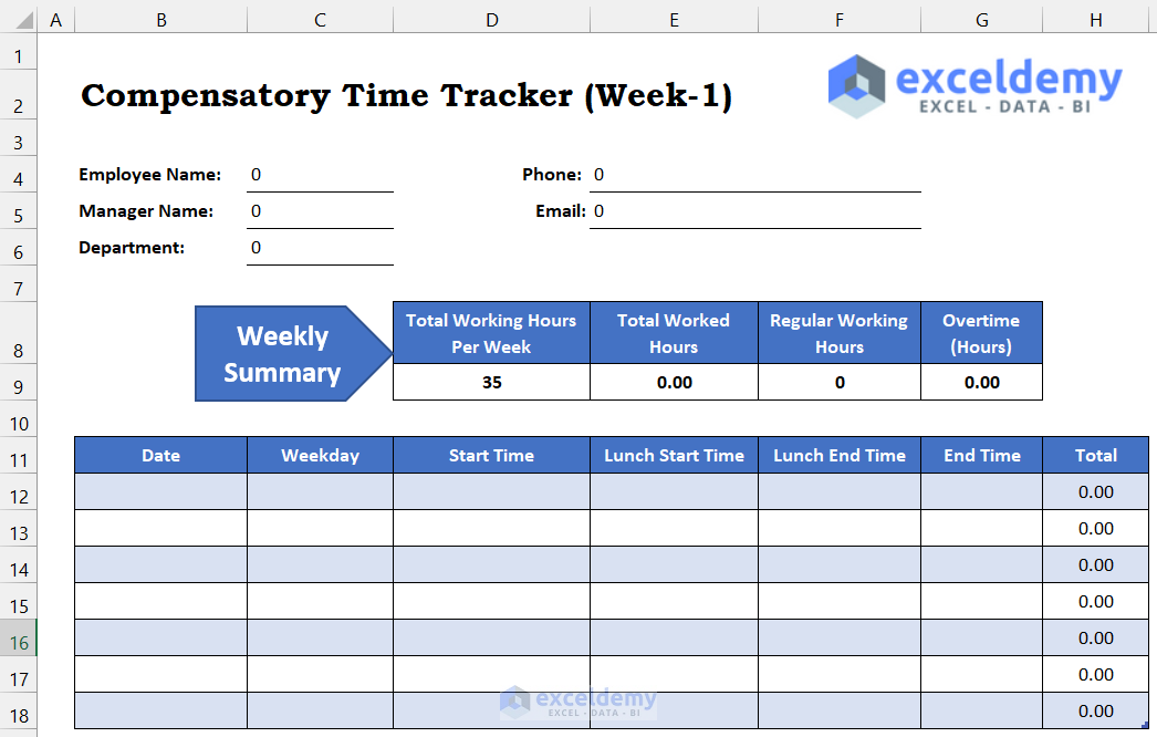
- Select cell B2 and change the sheet title Summary to Compensatory Time Tracker (Week-1).
Our weekly comp time tracking sheet for the first week is completed.
- Create four additional sheets for the rest of the days of that month.
- Input some sample data to check the accuracy of our formulas.
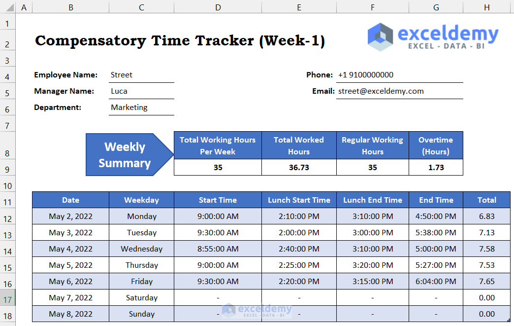
You will get the weekly summary report.
Breakdown of the Formula
We are breaking down the formula for cell C12.
We used the nested formula in cell C12 formula to get the weekday name. The formula is:
=IF([@Date]=0,” “,CHOOSE(WEEKDAY([@Date]),”Sunday”,”Monday”,”Tuesday”,”Wednesday”,”Thursday”,”Friday”,”Saturday”))
Now, we are breaking down the formula for cell C12.
WEEKDAY([@Date]: This function returns the sequential value of that weekday. For cell C12, the value is 2.
CHOOSE(WEEKDAY([@Date]),”Sunday”,”Monday”,”Tuesday”,”Wednesday”,”Thursday”,”Friday”,”Saturday”): This function will choose the day name. According to our formula, the value 2 represents Monday. As a result, the function returns Monday.
IF([@Date]=0,” “,CHOOSE(WEEKDAY([@Date]),”Sunday”,”Monday”,”Tuesday”,”Wednesday”,”Thursday”,”Friday”,”Saturday”)): The IF function first check the value of date column. If there is no value available in that column, the function will return space (“ “). Otherwise, it returns the weekday name, which it will get from the CHOOSE function. For the value of cell B12, the formula returns Monday.
Breakdown of the Formula
We are breaking down the formula for cell H12.
Similarly, we used another nested formula to get the total working hours of that day in column H.
=IFERROR(IF(COUNT(Comp_Time[@[Start Time]:[End Time]])=4,(IF([@[End Time]]<[@[Start Time]],1,0)+[@[End Time]])-[@[Lunch End Time]]+[@[Lunch Start Time]]-[@[Start Time]],IF(AND(LEN([@[Start Time]])<>0,LEN([@[End Time]])<>0),(IF([@[End Time]]<[@[Start Time]],1,0)+[@[End Time]])-[@[Start Time]],0))*24,0)
Now, we are breaking down the formula for cell H12.
IF([@[End Time]]<[@[Start Time]],1,0): This function returns 0.
LEN([@[Start Time]]: This function returns 12:00 AM.
COUNT(Comp_Time[@[Start Time]:[End Time]]): This function returns 4.
IF(AND(LEN([@[Start Time]])<>0,LEN([@[End Time]])<>0),(IF([@[End Time]]<[@[Start Time]],1,0)+[@[End Time]])-[@[Start Time]],0):This function returns 0.33.
AND(LEN([@[Start Time]])<>0,LEN([@[End Time]])<>0): This function returns TRUE.
IFERROR(IF(COUNT(Comp_Time[@[Start Time]:[End Time]])=4,(IF([@[End Time]]<[@[Start Time]],1,0)+[@[End Time]])-[@[Lunch End Time]]+[@[Lunch Start Time]]-[@[Start Time]],IF(AND(LEN([@[Start Time]])<>0,LEN([@[End Time]])<>0),(IF([@[End Time]]<[@[Start Time]],1,0)+[@[End Time]])-[@[Start Time]],0))*24,0): This formula returns the total working hours for that day. In this cell, the value is 6.83.
Read More: How to Design Employee Details Form in Excel
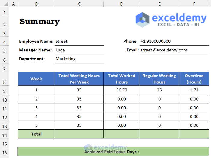
Step 3: Create a Summary Report
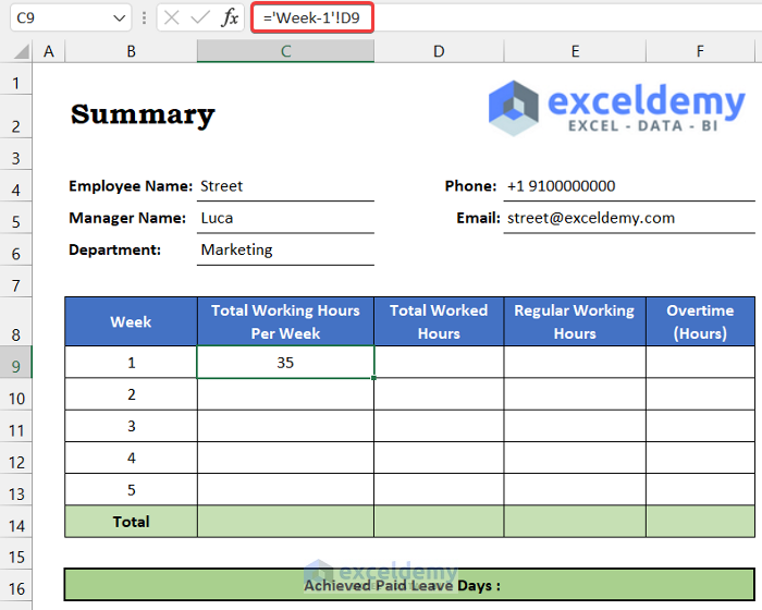
- Select cell C9 and enter the following formula into cells to get the value of the total working hours per week.
='Week-1'!D9
- Press Enter.
- Drag the Fill Handle icon to your right to copy the value-extracting formula up to cell F9.
- Insert the same formula to get the summary values for the rest of the weeks.
- To get the total, use the SUM function. Enter the following formula into cell C14:
=SUM(C9:C13)
- Press Enter.
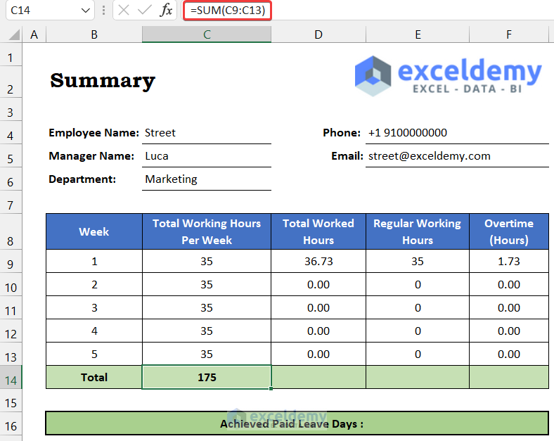
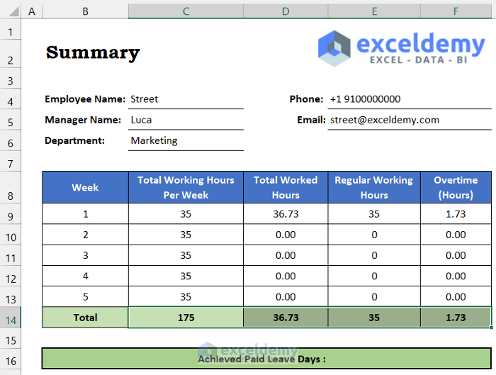
- Drag the Fill Handle icon to your right to get the total of all columns.
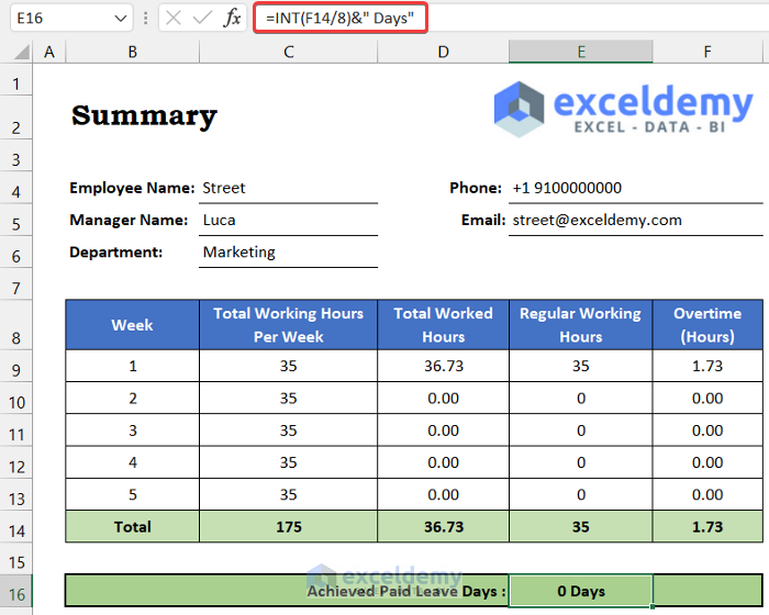
- To estimate the achievement paid on leave day, enter the following formula in cell E16. To get the complete day value, use the INT function.
=INT(F14/8)&" Days"
- Press Enter.
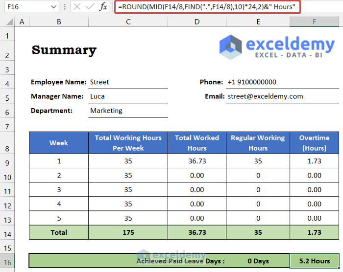
- You may notice in the manual calculation that our formula deducts the value after the decimal. To get that value in hour format, enter the following formula into cell F16 using the ROUND, MID, and FIND functions.
ROUND(MID(F14/8,FIND(".",F14/8),10)*24,2)&" Hours"
Breakdown of the Formula
We are breaking down the formula for cell F16.
FIND(“.”,F14/8): This function will search for the location of the decimal point in the result. In this value, the position of the decimal point is 2. As a result, the function returns 2.
MID(F14/8,FIND(“.”,F14/8),10): This formula will extract the value after the decimal point. We set the formula to extract 9 digits after the decimal. Thus, the function returns .21625.
ROUND(MID(F14/8,FIND(“.”,F14/8),10)*24,2)&” Hours”: Using this formula, we will get the final result. The function will round the value into 2 digits. So, the function will convert the value 1.73/8 or 0.22 into the hour. Hence, the function returns 5.2 Hours.
- Press Enter.
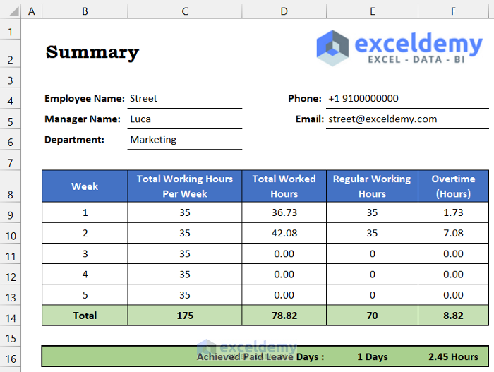
Our summary report is completed.
Step 4: Verify Comp Time Tracker with Data
- Input the employee details into the summary sheet.
- Input some sample data in the sheet named Week 2.

- You will get the summary report.
Read More: How to Create a Recruitment Tracker in Excel
Download the Practice Workbook
<< Go Back to Excel HR Templates | Excel Templates
Get FREE Advanced Excel Exercises with Solutions!
