How to Create a Recruitment Tracker in Excel: Step-by-Step Procedures

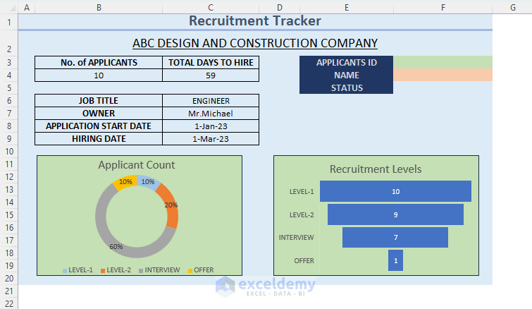
We are going to build a sample recruitment tracker template where you can search for a specific applicant and get the necessary information about them. Here is an overview of what our tracker dashboard looks like. The workbook contains three different sheets: Recruitment Tracker (Dashboard), Applicants Info (Information about the applicants are stored in a table of this sheet) and Recruitment Levels (Data to create charts are stored).

Step 1 – Making the Dataset for Recruitment Tracker in Excel

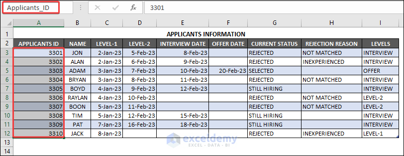
Here’s a sample dataset we will use for the recruitment tracker.

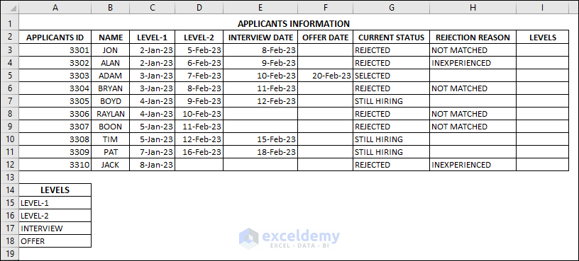
• Here, the recruitment process contains several levels of tasks such as Level-1, Level-2, and interview tasks. Each candidate needs to progress through them in order.
• Empty fields indicate that an applicant was rejected in the previous stage of the process.
• The interview date is assigned in the INTERVIEW DATE column. The OFFER DATE column contains dates for candidates who passed the process.
• The CURRENT STATUS column mentions whether a candidate is selected or rejected or if someone is considered to be hired in the future after the interview.
• The reasons for rejection of the rejected candidates in the interview are included in the REJECTION REASON column.
• We also made a helper column named LEVELS which will be helpful to develop formulas in the later sections.

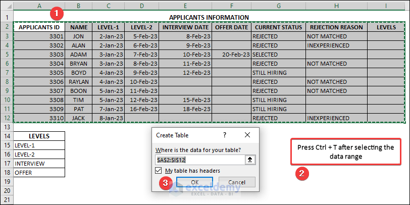
Now, we will convert this data range to an Excel table because Excel table is dynamic to use. Whenever you add a new row to your data range, the table will automatically calculate apply the formulas and formatting.

• Select the data range and press Ctrl + T.
• A dialog box will pop up showing the cell range for the table.
• Select ‘My table has headers‘ and click OK.

• Select any cell on the table and then choose the Table Design tab.
• Go to Table Styles Options and uncheck the Filter Button.

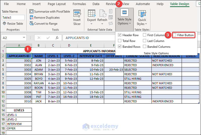
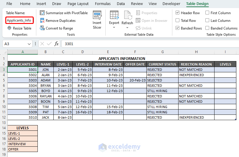
You can see that the Filter buttons are now gone. You can also choose your own table design from the Table Styles group.

• Give a suitable name for the table. This name can be used to use the table anywhere in the workbook. You can input the name for the table in the Properties group of the Table Design tab.

Step 2 – Generating Formula to Setup Necessary Parameters

If someone passes level-2 and proceeds to the interview, the formula will return “INTERVIEW“. If someone passes the level-2 but doesn’t succeed the interview, the result will be “LEVEL-2“. This employs that the candidate passed the level-1 tasks.

Use this formula:

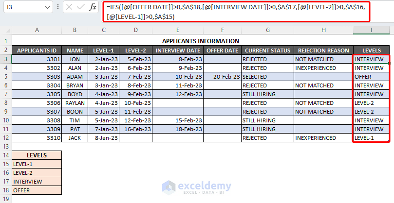
Step 3 – Creating and Formatting Dynamic Charts for Recruitment Tracker Dashboard

Let’s create a dynamic recruitment tracker by creating an applicant pipeline.

Use the formula below with the COUNTIF function to find out the number of applicants who failed in a particular stage. We stored the counts in the Applicant Count column.

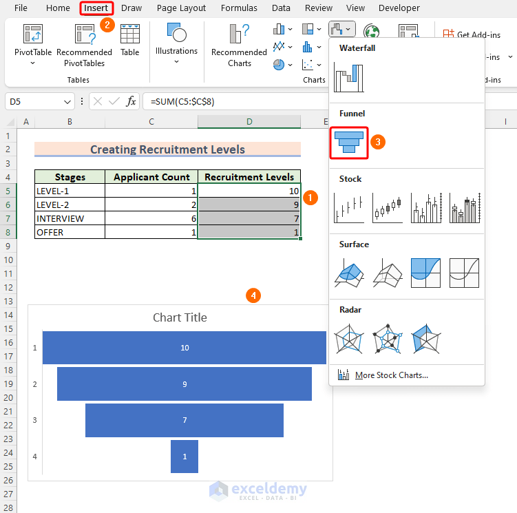
And the following formula sums up the total number of candidates who attended a particular stage. We stored this data in the Recruitment Levels column.

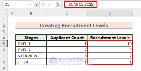
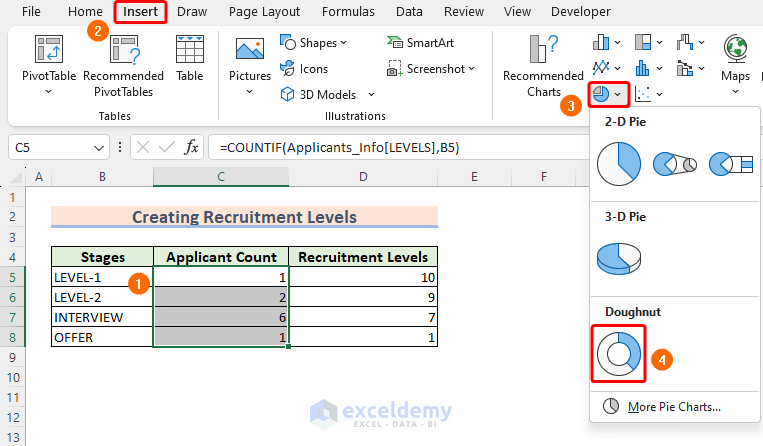
To visualize the data of Applicant Count and Recruitment Levels columns, we will create a Doughnut Chart and a Funnel Chart respectively:

• Select the cell range C5:C8 and choose the Insert tab.
• Go to Doughnut Chart from the Insert Doughnut or Pie Chart group.

• Remove Fill Color from the chart background.
• Right-click on the current Axis Labels and select ‘Select Data’ from the Context Menu. The Select Data Source dialog box will appear.
• Click on the Edit button under the Horizontal (Category) Axis Labels.
• Select the data range B5:B8 to insert the data of the Stages column as labels and click OK. You will see them in the Axis Labels.

You can also change the fill color of a specific portion of your chart. Suppose we want to change the fill color of the blue portion of the chart. To do that:

• Select the portion first. It may take some time if your chart is small, so drag out the chart to make it bigger.
• Right-click on it, select Fill, and choose a color.

This will change the fill color of the specific part of the doughnut chart. Moreover, you can change or modify the appearance of the chart using the options from the Chart Design tab. There are various options for formatting charts.

Now we need to create a Funnel Chart which will show the number of total applicants in a specific level.

Go to Insert, click on the Chart option, and select Funnel.

Change the Axis Labels following the procedure described for the Doughnut Chart.

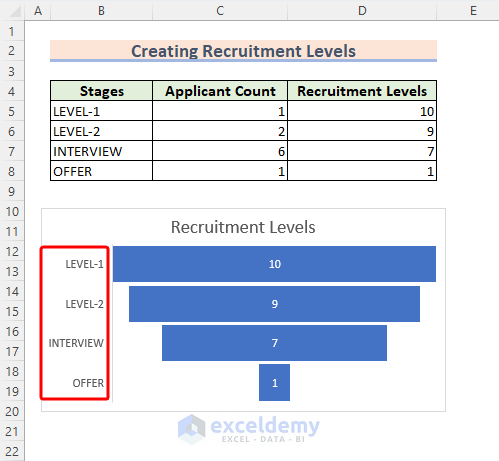
The Funnel Chart has meaningful axis labels now.

Read More: How to Track Comp Time in Excel

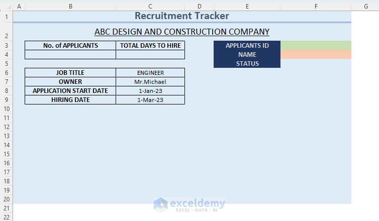
Step 4 – Setting Up Recruitment Tracker Dashboard

• Pick some cells to store the necessary data you want to display in the dashboard. We typed necessary headings here and used different fill color for the Applicants Data.

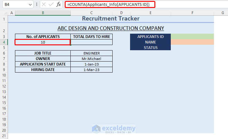
• To count the total number of applicants, use the formula below:

The formula uses the COUNTA function to count how many applicants attended for the job. The advantage of using the COUNTA function is that it doesn’t count blank cells.

• The following formula returns the total number of days of the hiring process:

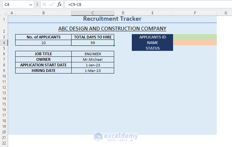
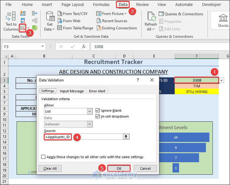
Let’s apply a Data Validation list for the Applicants IDs:

• Select a cell to store the list, go to Data, and then to Data Validation.
• In the Data Validation dialog box, select List under the Allow drop-down.

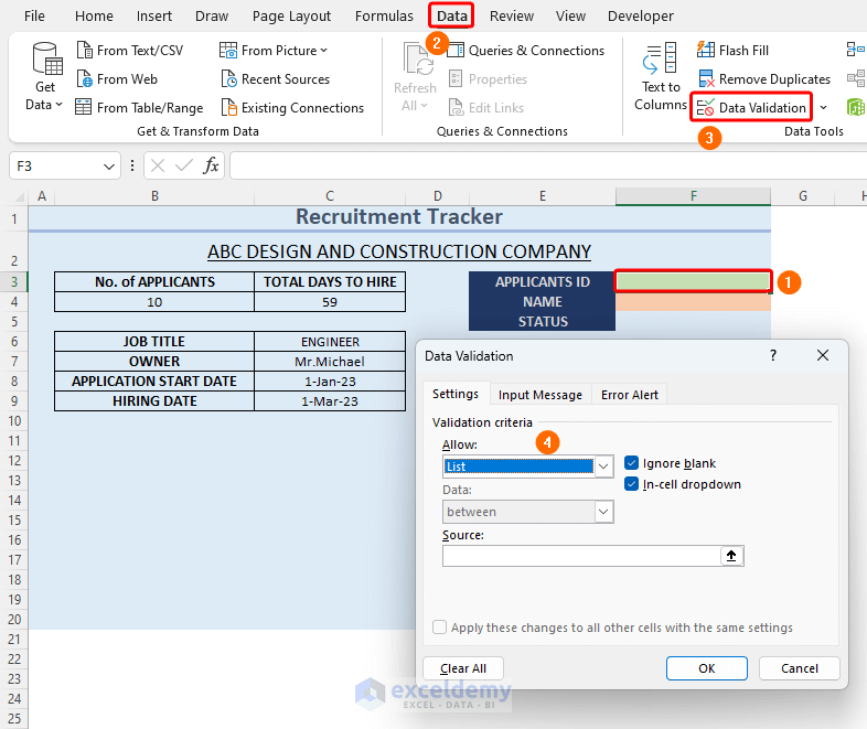
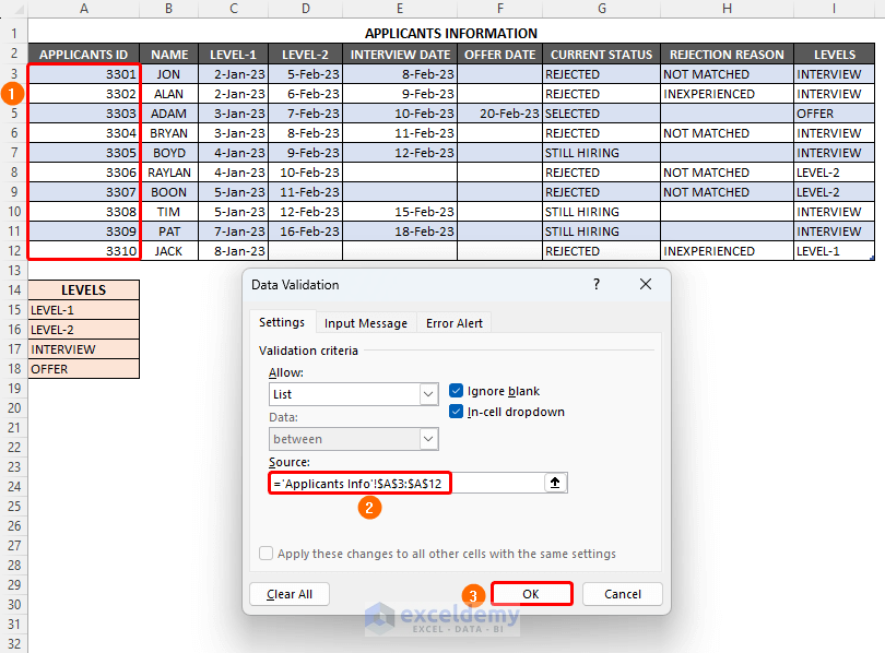
• Select the data range containing Applicants IDs (A3:A12 in the Applicants Info sheet) for the Source.
• Click on OK.

• Paste the following formula in F4 to return a name corresponding to the selected ID. It uses the VLOOKUP function to search for the ID selected in the F3 cell in the Applicants_Info table and return the name from its NAME column. The IFERROR function is used to ignore the error which can occur from the absence of data in cell F3.

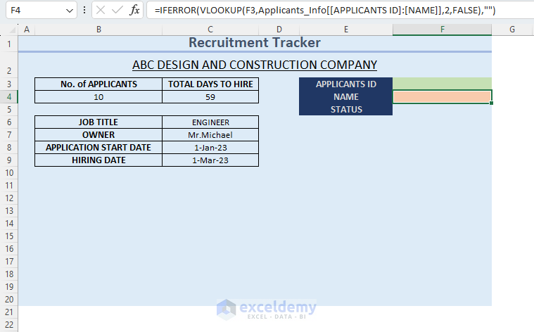
• In F5, put the following formula to retrieve the status of the candidate.

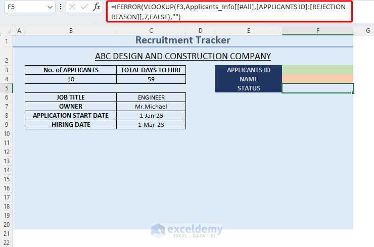
• Copy the following formula into E6 to generate row header based on the cell value in F5.

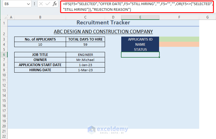
If the STATUS is SELECTED, the formula returns “OFFER DATE”. If it is “STILL HIRING”, then the formula returns blank. The formula also returns “REJECTION REASON” if the value of cell F5 is neither “SELECTED” nor “STILL HIRING”.

• Put the following formula into F6, which returns REJECTION REASON or OFFER DATE for the corresponding applicant based on the value of cell E6.

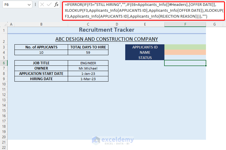
The formula uses the XLOOKUP function to return the REJECTION REASON or OFFER DATE from the Applicants_Info table. It will return blank if the cell value of F5 is “STILL HIRING”.

Let’s format the table a bit:

• Go to Insert and select Shapes.
• Choose the rectangular shape.

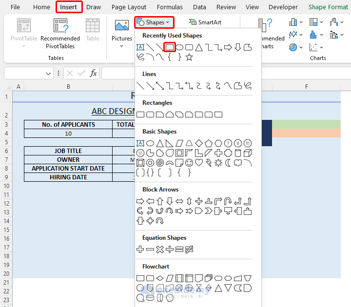
• Hold the mouse button and drag it to draw the rectangles in the table.
• Hold the Ctrl button and drag the created shape around to copy it.
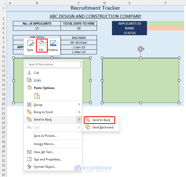
• Select both of the shapes and right-click on any of them.
• Go to “Fill” and choose a fill color.
• Select Send to Back and Send to Back again to make the shape into a background of the chart.

• Copy the charts from the Recruitment Levels sheet, paste them, and place them on the rectangles.

Now, the charts have a better view to visualize for the users.

Step 5 – Using the Dashboard

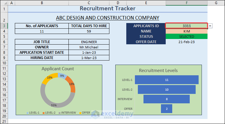
• Click on the Applicants ID drop-down (cell F3).
• Select an ID from the drop-down list.
• The corresponding names, statuses, and rejection reasons/offer dates will appear automatically.

Step 6 – Applying Conditional Formatting Feature to Dashboard

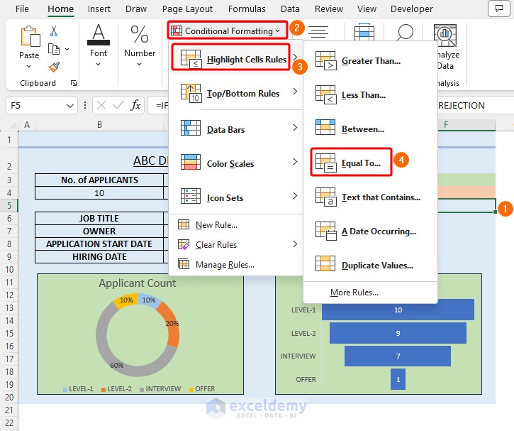
• Select the cell containing the data of the applicants’ status and choose Conditional Formatting.
• Go to Highlight Cell Rules.
• Select Equal To… A dialog box named Equal To will pop up.

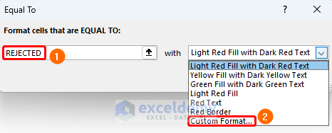
• Type REJECTED in the Format cells that are EQUAL TO section and choose Custom Format from the drop-down on the right.

• We chose the Red color for the REJECTED status.

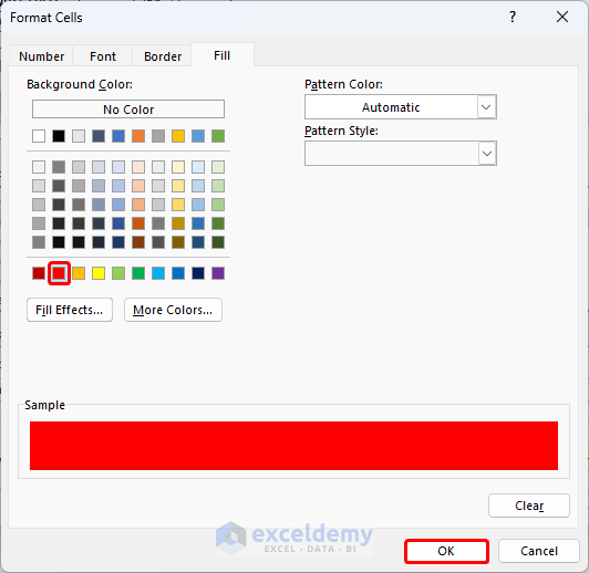
• Repeat the process for SELECTED and STILL HIRING. We chose green and yellow colors for the SELECTED and STILL HIRING statuses, respectively.

You will now see different background colors based on applicant status.

Step 7 – Adding Named Range to Make Recruitment Tracker Template Dynamic

Say you insert a new candidate information in the Applicants_Info table. If you search for the new entry in the drop-down list of IDs, you won’t find it. That’s why we need a named range for the Applicants IDs:

• Select the cell range (A3:A12) and type a name in the Name Box. We used Applicants_ID.

• Replace the source of the Data Validation list with this named range.

• Add a new entry. Here, we inserted an applicant named “KIM” and their other information.

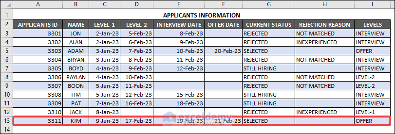
You will find the drop-down list updated with the new ID, and selecting this will retrieve corresponding information about her.

Read More: How to Design Employee Details Form in Excel

Download Free Template

<< Go Back to Excel HR Templates | Excel Templates