Method 1 – Calculate Standard Deviation with Single IF Condition
Steps:
- Select the desired cell where we want to get the result as shown in the image below.
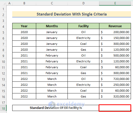
- Enter the following formula below.
=STDEV(IF(D5:D16="Oil",E5:E16))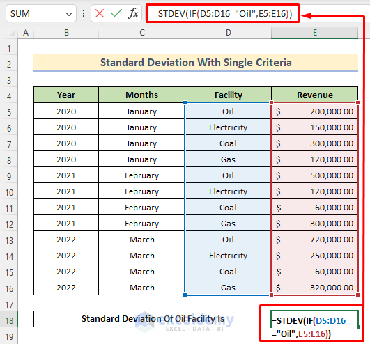
Formula Breakdown
- The IF(D5:D16=”Oil”,E5:E16) returns only the values of Revenue that are based on criteria D5:D16=”Oil”. We will get only the revenues from the Oil
- The D column or the Facility column is the criteria for choosing the dataset. The E column or the Revenue column is the data range-making column. You can use your own data range and choose criteria according to your needs.
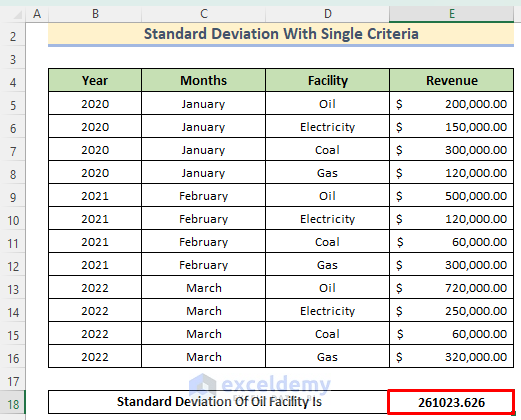
- The STDEV will find out the standard deviation of the selected data set by the IF function. We will get the standard deviation of revenue only from the oil facility.
- Press Enter to get the result.
Read More: How to Calculate Standard Deviation of y Intercept in Excel
Method 2 – Calculate Standard Deviation with Multiple IF Conditions
Steps:
- Select the destination cell.
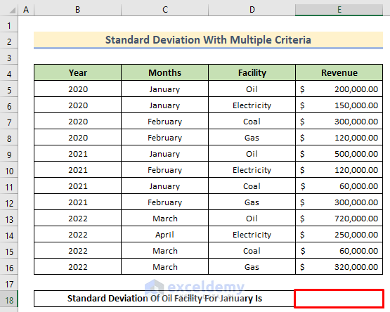
- Enter the following formula below.
=STDEV(IF((C5:C16="January")*(D5:D16="Oil"),E5:E16,""))
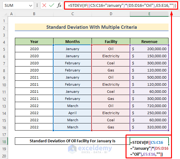
Formula Breakdown
- The =STDEV() function is to find out the standard deviation.
- The IF function is to select the data range based on criteria.
- We needed the data of month January and facility Oil. So, by entering (C5:C16=”January”)*(D5:D16=”Oil”), we defined the cell range and multiplied these two criteria as these conditions are dependent on finding the value.
- We entered the range values we need to select from, that being E5:E16.
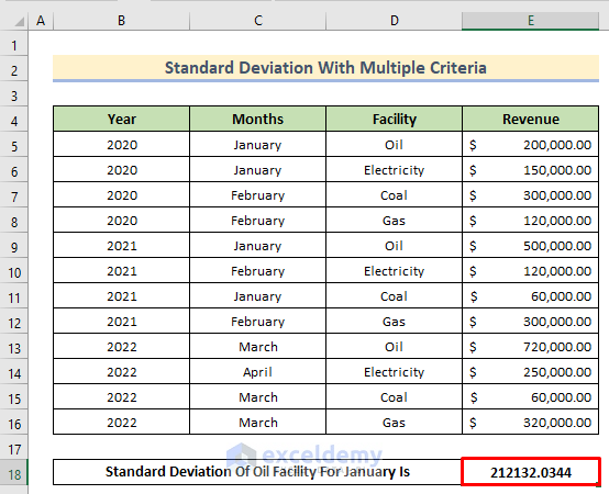
- Combine them to get a standard deviation based on multiple criteria.
- Press Enter to get the expected result.
Read More: How to Calculate Population Standard Deviation in Excel
Download Practice Workbook
Related Articles
- How to Calculate Standard Deviation of a Frequency Distribution in Excel
- Calculate Percentile from Mean and Standard Deviation in Excel
- How to Calculate Uncertainty in Excel
- How to Calculate Mean and Standard Deviation in Excel
<< Go Back to Standard Deviation Formula in Excel | Excel for Statistics | Learn Excel
Get FREE Advanced Excel Exercises with Solutions!

this methood is worng since it take all the fulse as 0
and + need to use CTRL+SHIFT+ENTER
Dear AVI,
We can assure you that if you followed the steps correctly, everything should be fine with the tutorial. Moreover, both of these formulas are single-cell output formula. So, the procedure for the array formula implementation or pressing CTRL+SHIFT+ENTER is not required here.
If you want to take all the data to find out the standard deviation without conditions or avoid taking the false as 0, you should have a look at our article How to Calculate Average and Standard Deviation in Excel.
Regards,
Exceldemy
Hi,
A couple of questions relating to the above formulae and explanation:
1) why does the formula for multiple IFs include “” at the end?
2) when does the criteria need to be in quotation marks? my computation of an SD with one condition doesn’t work if these are included, but does if they are excluded.
3) using your formula for multiple IFs i continually get an error dialogue box. However, when i use the below – eventually- it works
=STDEV(IF((S2:S295>=-6)*(K2:K295=1),F2:F295))
thanks
Hello Jeremy,
1. The “” at the end of the formula in the article is the value_if_false for the IF function. It ensures that when a row does not meet the criteria, an empty string is returned, which STDEV.S ignores in the calculation.
2. Criteria need to be in quotes when you are testing for text values or when using operators inside functions like SUMIFS. For numbers in an IF condition, do not use quotes (for example, S2:S295>=-6). For text, quotes are required (for example, K2:K295=”Yes”).
3. If the multiple IFs formula gives an error, common reasons are:
3.1. The ranges are not the same size.
3.2. In older versions of Excel, the formula is not entered as an array formula using Ctrl+Shift+Enter.
3.3. Your Excel version uses semicolons instead of commas as list separators.
The formula you provided:
=STDEV.S(IF((S2:S295>=-6)*(K2:K295=1),F2:F295))
It works correctly for the AND condition explained in the article. In Excel 365, you can also use:
=STDEV.S(FILTER(F2:F295,(S2:S295>=-6)*(K2:K295=1)))
Hope this clarifies your queries.
Regards
ExcelDemy