Method 1 – Find y Intercept to Calculate Standard Deviation in Excel
Find the y-intercept of the given dataset. We can use various functions to find the y-intercept in Excel.
Find the y-intercept by simply using the INTERCEPT function in Excel. Follow the steps below:
- Select a cell where you want to see the y-intercept. We are selecting cell C19 to see the y-intercept for the first quarter. Enter the following formula into the cell:
=INTERCEPT(D5:D8,C5:C8)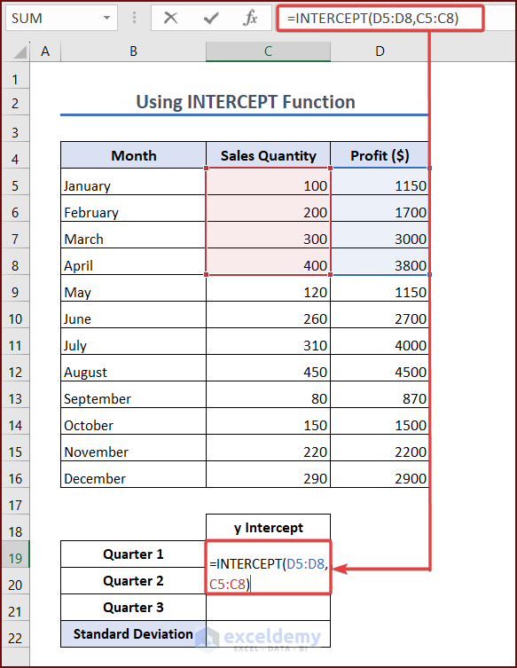
- Press Enter and you will see the y-intercept for the first quarter in cell C19. Enter the following formulae in cells C20 and C21 to get the y-intercepts for the second and third quarters, respectively:
=INTERCEPT(D9:D12,C9:C12)=INTERCEPT(D13:D16,C13:C16)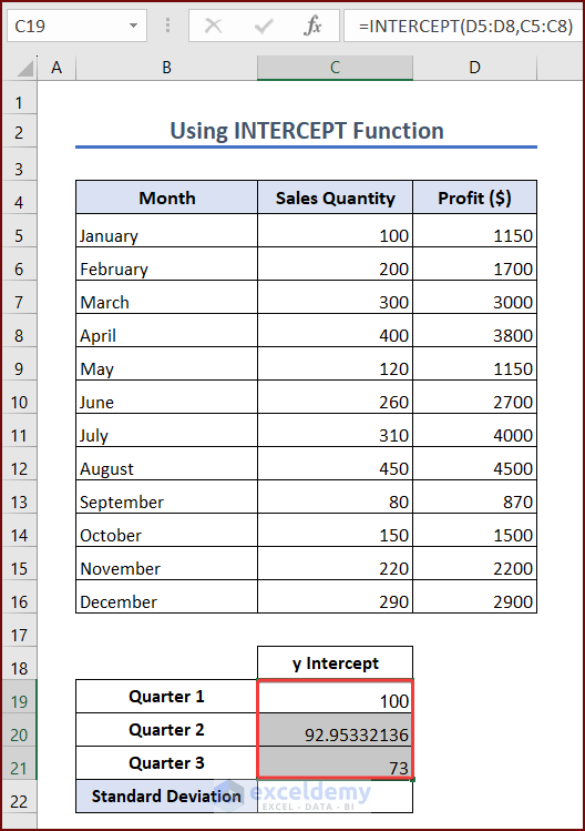
Method 2 – Combine AVERAGE and SLOPE Functions
Combine the AVERAGE and SLOPE functions to calculate the y intercept. Follow these steps:
- Select cell C19 to see the y-intercept for the first quarter. Enter the following formula into the cell:
=AVERAGE(D5:D8)-SLOPE(D5:D8,C5:C8)*AVERAGE(C5:C8)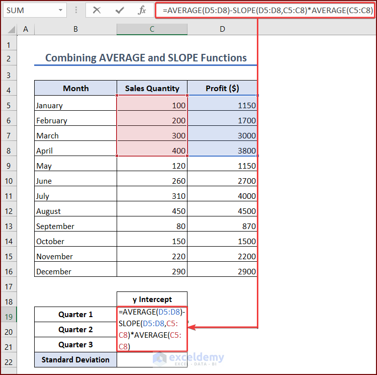
Formula Breakdown
- AVERAGE(D5:D8): We used the AVERAGE This function will take the values of cells D5:D8 and will calculate the arithmetic mean or average of these values accordingly.
- SLOPE(D5:D8,C5:C8): The SLOPE function takes two inputs. The first input is the range of cells representing y values, and the second is the range of cells representing x values. This function returns the slope of the input data points.
- AVERAGE(D5:D8)-SLOPE(D5:D8,C5:C8)*AVERAGE(C5:C8): This whole formula calculates the y-intercept of the input data points.
- Press Enter, and see the y-intercept for the first quarter in cell C19. Enter the following formulae in cells C20 and C21 to get the y-intercepts for the second and third quarters:
=AVERAGE(D9:D12)-SLOPE(D9:D12,C9:C12)*AVERAGE(C9:C12)=AVERAGE(D13:D16)-SLOPE(D13:D16,C13:C16)*AVERAGE(C13:C16)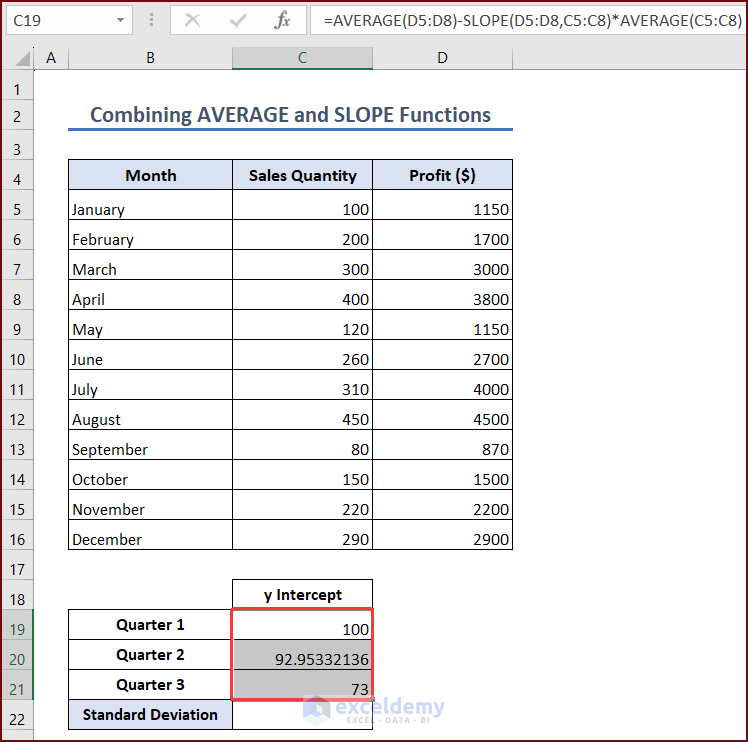
Method 3 – Use the LINEST Function
Use the LINEST function to find the value of the y-intercept in Excel. The LINEST is an array formula. Returns multiple outputs, and each output signifies different values. Follow the steps below:
- Select cell C19 and enter the formula into the cell:
=LINEST(D5:D8,C5:C8)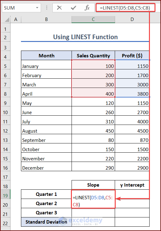
- Press Enter, and the LINEST function will return two values in two consecutive cells. The first is the slope, and the second is the y-intercept. The y-intercept for the first quarter will be in cell D19.
- Enter the following formulae in cells C20 and C21. You will get the y-intercepts for the second and third quarters in cells D20 and D21:
=LINEST(D9:D12,C9:C12)=LINEST(D13:D16,C13:C16)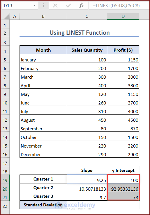
Method 4 – Using STDEV and STDEV.S Functions to Calculate Standard Deviation of y Intercept in Excel
1. Use STDEV Function
Use the STDEV function to calculate the standard deviation of the y-intercept in Excel. This formula is compatible with Excel 2007 and earlier. Follow the steps below:
- Select a cell where you want to see the standard deviation of the y-intercept. We are selecting cell C22. Enter the formula into the cell:
=STDEV(C19:C21)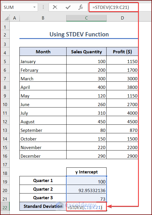
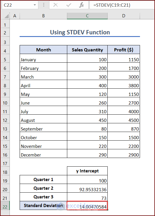
- Press Enter, and you will see the standard deviation of the y-intercept in cell C22.
2. Use STDEV.S Function
Use the STDEV.S function to calculate the standard deviation of the y-intercept. Just follow these steps:
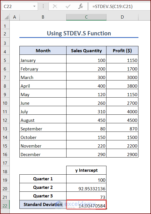
- Select a cell where you want to see the standard deviation of the y-intercept. We are selecting cell C22. Enter the formula into the cell:
=STDEV.S(C19:C21)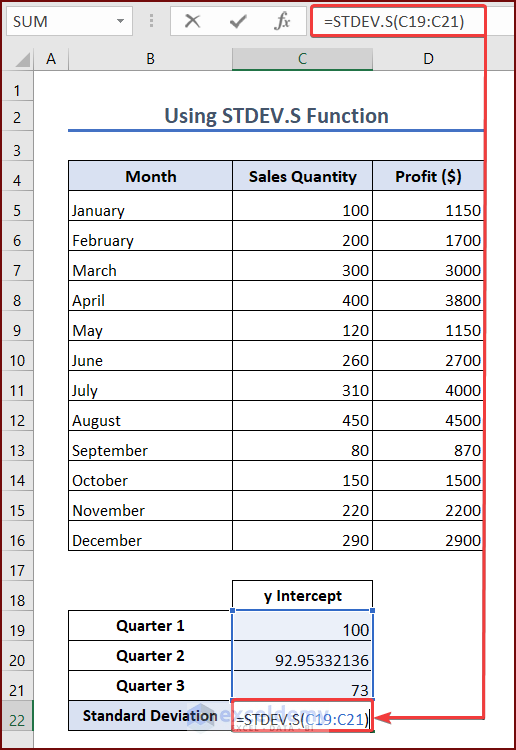
- Press Enter, and you will see the standard deviation of the y-intercept in cell C22.
Error in Intercept in Excel
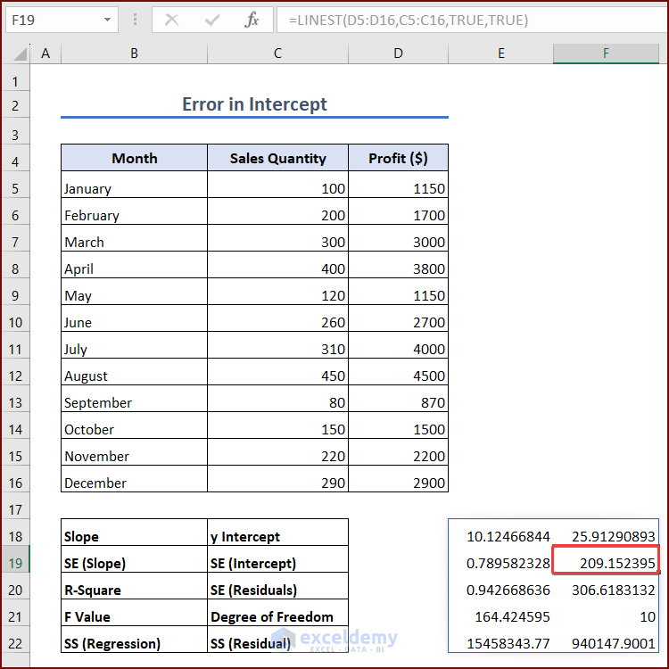
- Select a cell to enter the formula. We are selecting cell E18:
=LINEST(D5:D16,C5:C16,TRUE,TRUE)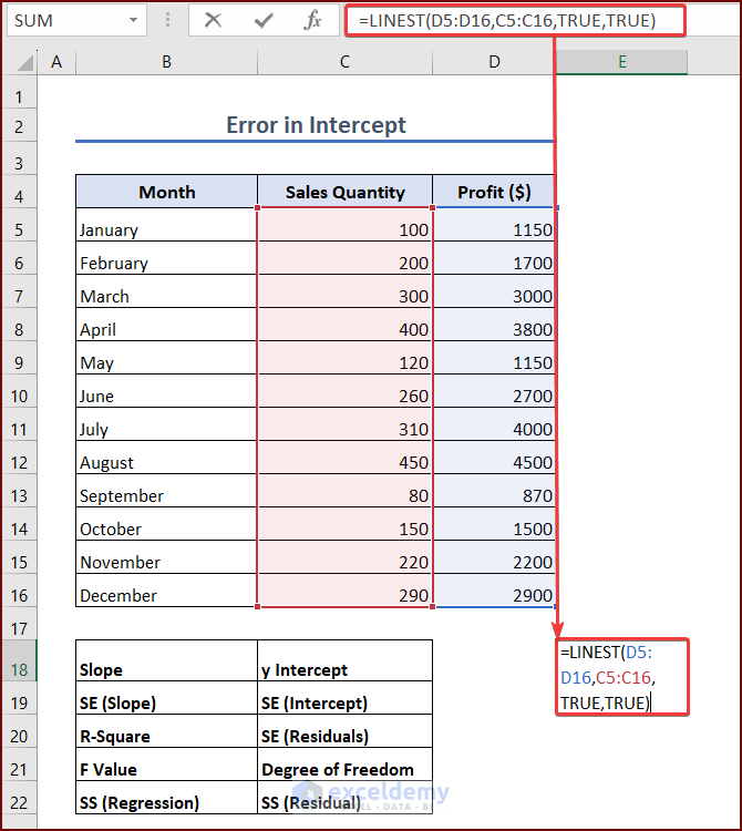
- Press Enter, and you will see an array of outputs. Cells B18:C22 represent the output values of cells E18: F22. It is visible that the standard error of y-intercept is the value in cell F19.
Things to Remember
There are a few things to remember while calculating the standard deviation of the y-intercept in Excel:
- Use the correct formula. If the data set is a sample dataset, use S and if it is a population dataset use the STDEV.P function.
- The LINEST function returns multiple outputs. Carefully choose the value you want from the array of outputs.
Frequently Asked Questions
1. What does a high or low standard deviation mean?
A high standard deviation indicates that the data points are spread out widely from the mean, whereas a low standard deviation means that the data points are clustered closely around the mean.
2. Can the standard deviation be negative?
No, the standard deviation cannot be negative. It is always either a positive number or zero.
3. Can the standard deviation be greater than the mean?
Yes, the standard deviation can be greater than the mean if the data points are spread out widely from the mean.
Download Practice Workbook
You can download the practice workbook while going through this article.
Related Articles
- How to Calculate Standard Deviation of a Frequency Distribution in Excel
- Calculate Percentile from Mean and Standard Deviation in Excel
- How to Calculate Uncertainty in Excel


Hi,
I have a question. I see that you used the “standard error” directly as “standard deviation of the y intercept”. I think they are different terms, so strictly speaking, are they supposed to be different values?
Thanks.
Hello Z L
Thank you very much for your response. We have modified this article and introduced some new statistical concepts and functions. Would you please go through it again?
If you have any more questions, let us know in the comment section.
Thanks
Md. Abu Sina Ibne Albaruni
Team ExcelDemy