How to Sort Rows in Excel (3 Easy Ways)

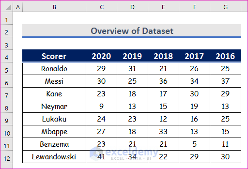
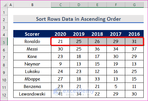
To demonstrate methods for sorting rows in Excel, we’ll utilize this simple dataset listing several footballers and their goals scored over the last five seasons.

Method 1 – Using Excel Sorting Tools to Sort Rows Without Mixing Data

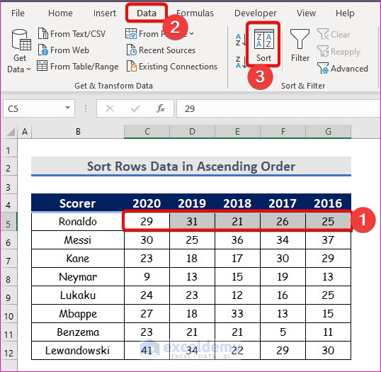
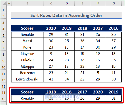
Case 1.1 – Sort Rows in Ascending Order

Step 1:

Select the row you want to sort. We will select the data range from C5 to C12.
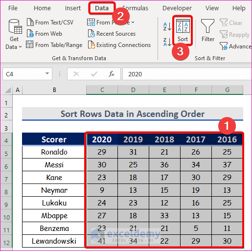
From the Data tab, Sort & Filter and choose Sort.

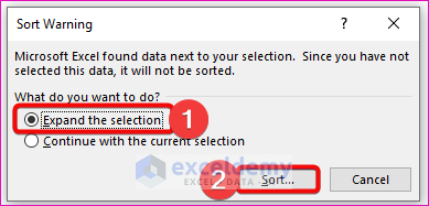
Since only one row has been selected from the table, Excel will show the Sort Warning dialog box. Select Expand the selection and click Sort.

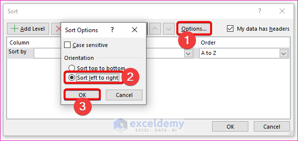
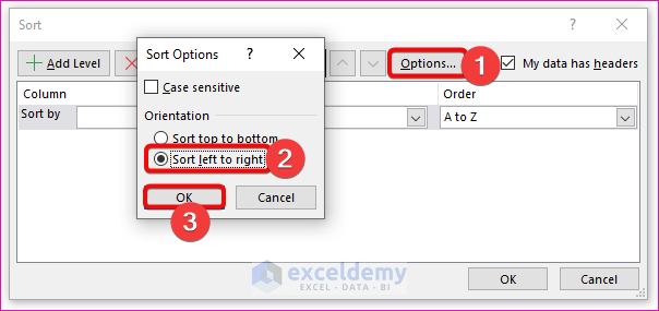
The Sort dialog box will pop up. Click Options from the dialog box, which will open a new dialog box, Sort Options.
Select Sort left to right and click OK.

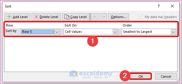
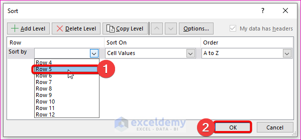
In the Sort by dialog box, the names of the rows appear. Select your preferred row (we have selected Row 5) and click OK.

The row is sorted in ascending order.

Step 2:

To prevent the index column (Scorer) from changing position:

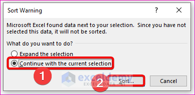
Go back to the Sort Warning dialog box and select Continue with the current selection.
Press Sort.

If we explicitly select a particular row, then we don’t need to select Sort left to right from the Options. The row will be pre-selected in the Sort dialog box.

Click OK. The row will be sorted in ascending order.

Step 3:

The data is not organized correctly. Select the columns associated with the row we are going to sort.

Click Sort, then Options in the Sort dialog, then select Sort left to right and click OK.

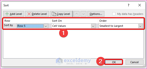
Select the desired row from the drop-down list of rows and click OK.

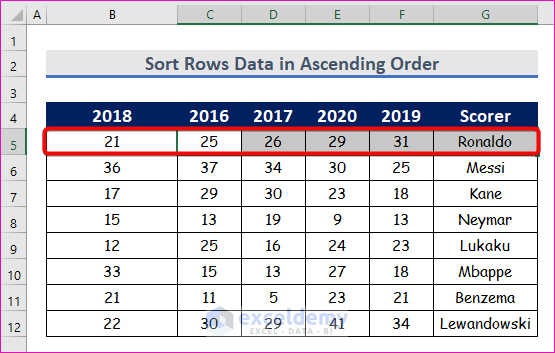
Row 5 (our selected row) has been sorted in ascending order. For illustrative purposes, the sorted output is shown separately, but the result will usually appear within the table itself.

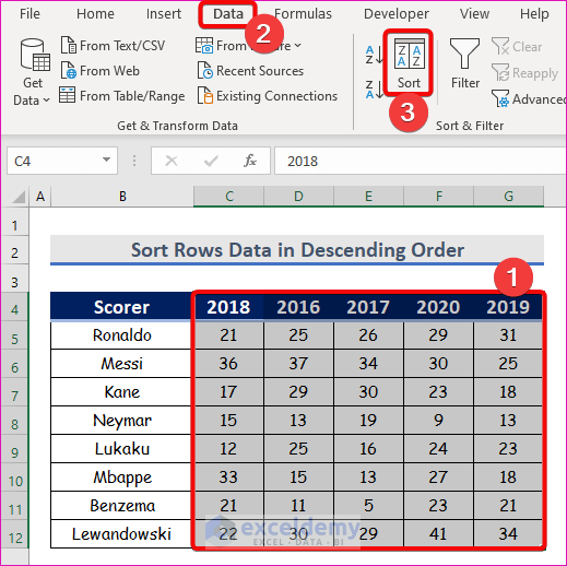
Case 1.2 – Sort Rows Data in Descending Order

Steps:

Select the rows and columns as before and click Sort.
Select the Sort left to right from the Options in the Sort box and click OK.

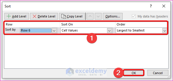
Select the desired row from the Sort by list, then select Largest to Smallest from the Order drop-down list of options and click OK.

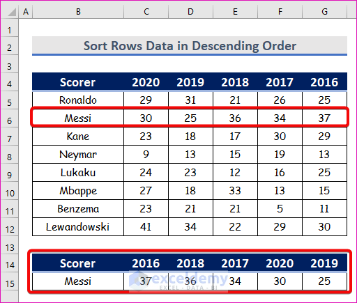
This time we selected Row 6, which has been sorted in descending order. To illustrate, the result is again shown separately.

Similar Readings

Method 2 – Sort Rows Using Formulas in Excel

Case 2.1 – Applying the SMALL Function to Sort in Ascending Order

Steps:

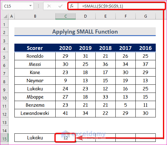
Determine the smallest value using the formula

=SMALL($C$9:$G$9,1)

We are using Row 9. The second argument is 1 so that we get the lowest value in this row.

12 is the smallest value in the row, and is correctly returned by the formula.

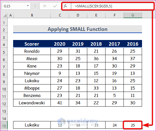
Change the number in the parameter of the SMALL function to find the other values in ascending order. Here we use values 1 to 5 since our row has 5 values.

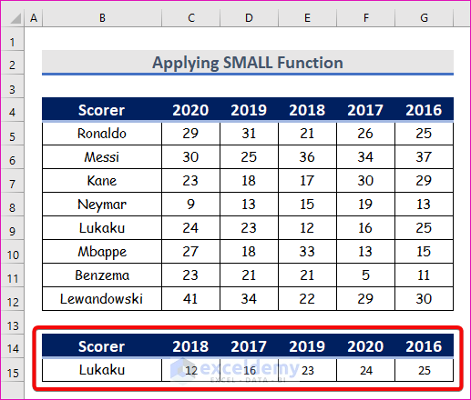
The row is sorted in ascending order, but we have to set the heading and the athlete’s name manually.

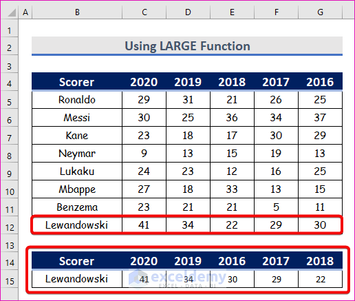
Case 2.2 – Using the LARGE Function to Sort in Descending Order

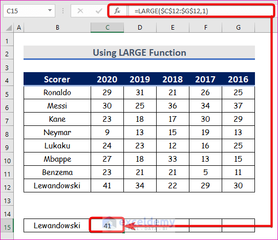
To find the highest value in the row, use the following formula:

=LARGE($C$12:$G$12,1)

This formula returns the highest value from Row 12.

Now change the number in the second parameter of the LARGE function to retrieve the second highest, third highest, and so on. We use the values 1 to 5 since the row has 5 numbers in it.

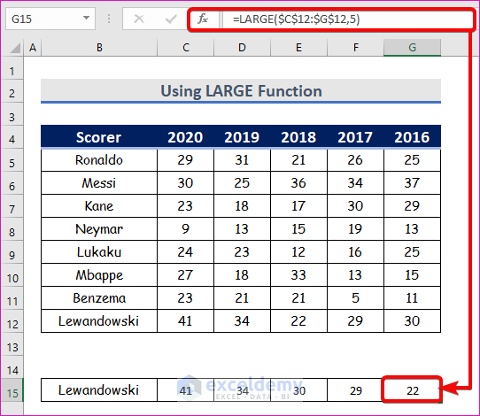
The row is sorted in descending order. We have to set the heading and the athlete name manually.

Caution

This method of sorting can be problematic since the heading must be set manually and when you have a bunch of data, some of them can be returned in the wrong column(s).

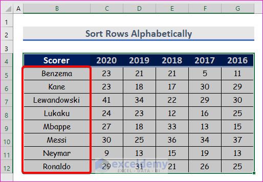
Method 3 – Sort Rows Alphabetically and Keep Rows Together in Excel

Steps:

Select the data range from B4 to G12.
From the Data tab, select Sort & Filter and pick Sort.

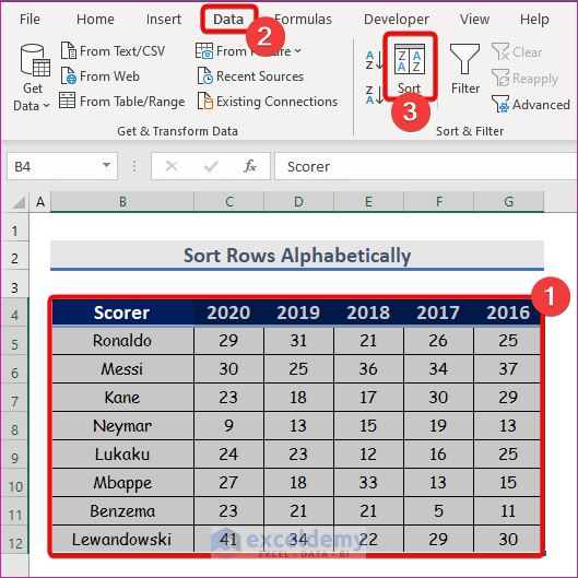
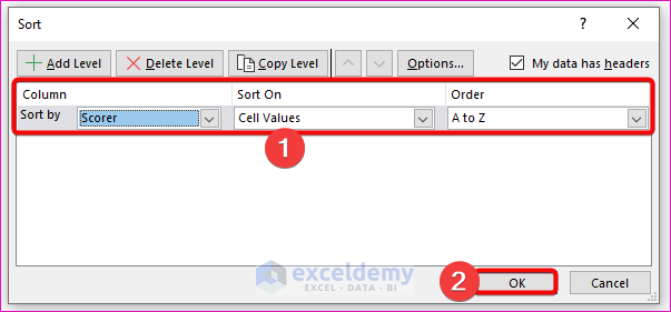
The Sort dialog box opens. Select Scorer from the Sort by drop-down list, then Cell Values from the Sort On drop-down list, and A to Z from the Order drop-down list.
Press OK.