How to Sort Column by Value in Excel (7 Easy Ways)

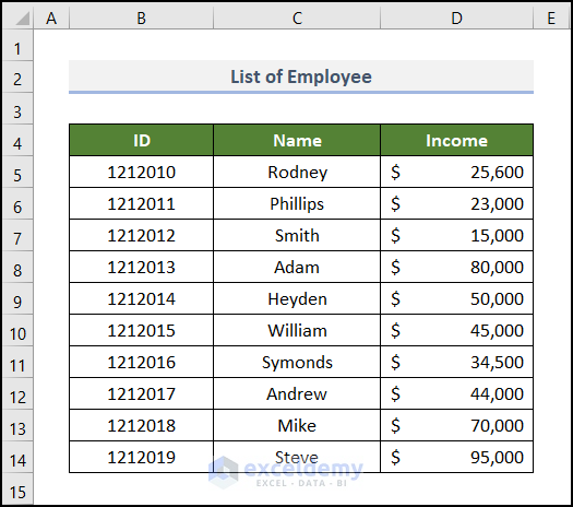
Let’s use a List of Employees. This dataset includes the IDs, Names, and their corresponding Income in columns B, C, and D, respectively. We’ll use it to sort the columns by some values.

Method 1 – Using Quick Sort Commands

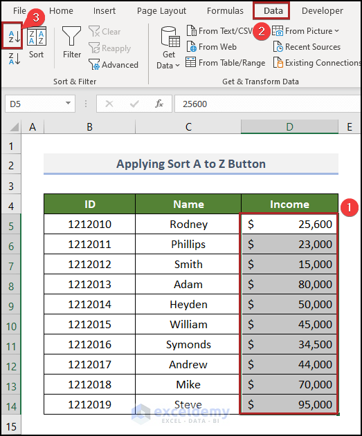
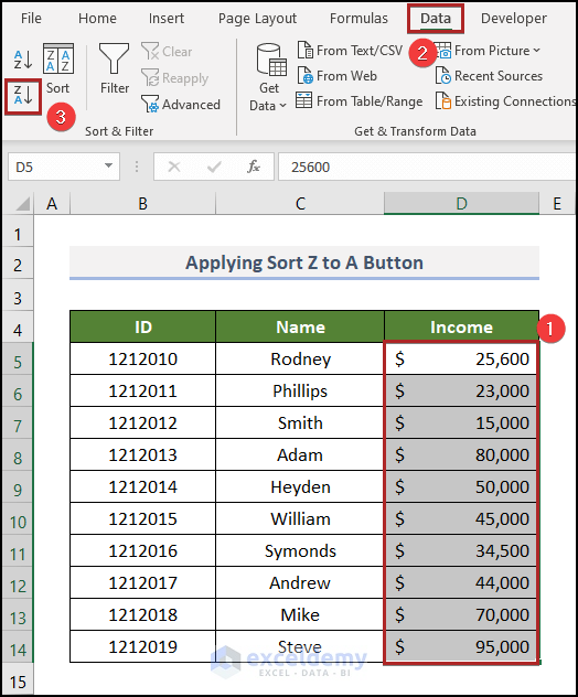
Case 1.1 – Applying the Sort A to Z Button

Steps:

• Select the cells in the D5:D14 range.
• Go to the Data tab.
• Click on the Sort A to Z icon on the Sort & Filter group of commands.

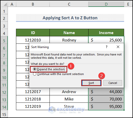
• The Sort Warning dialog box appears. Click on Expand the selection under the What do you want to do? section.
• Click on Sort.

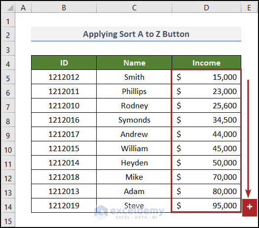
• Our columns are sorted from smallest to largest.

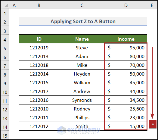
Case 1.2 – Applying the Sort Z to A Button

Steps:

• Select the data in the Income column.
• Move to the Data tab.
• Click on the Sort Z to A icon.

• Expand the selection in the warning box and confirm.

Read More: How to Sort Two Columns in Excel to Match

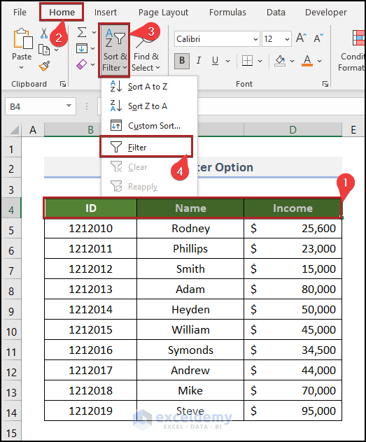
Method 2 – Utilizing the Filter Option

Steps:

• Select all the column headings in the B4:D4 range.
• Go to the Home tab.
• Click on the Sort & Filter drop-down on the Editing group.
• From the drop-down list, select the Filter option.

• The filter button is available next to each column heading.

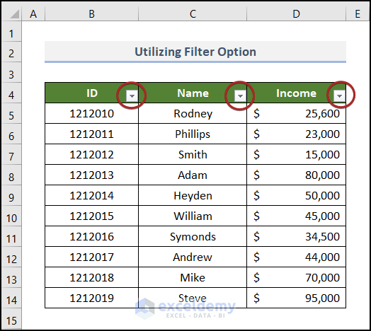
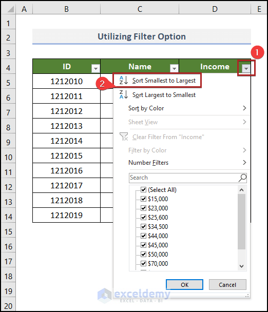
• Click on the filter button of the Income column.
• Select Sort Smallest to Largest from the options.

• We can see the columns get sorted from the smallest to the largest value.

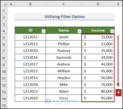
• Similarly, you can sort from largest to smallest.

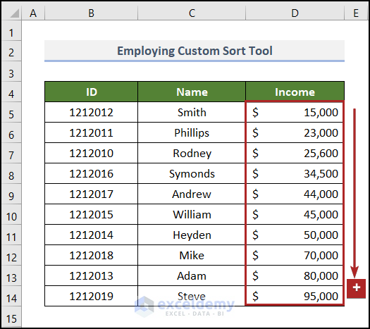
Method 3 – Using a Custom Sort Tool

Steps:

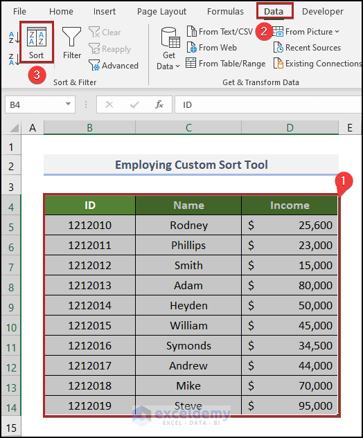
• Select cells in the B4:D14 range.
• Go to the Data tab.
• Click on the Sort icon on the Sort & Filter group.

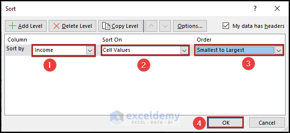
• The Sort wizard pops up. Here you can customize your sorting styles. We will Sort by the Income column, Sort On the Cell Values, and the Order is Smallest to Largest.
• Click on OK.

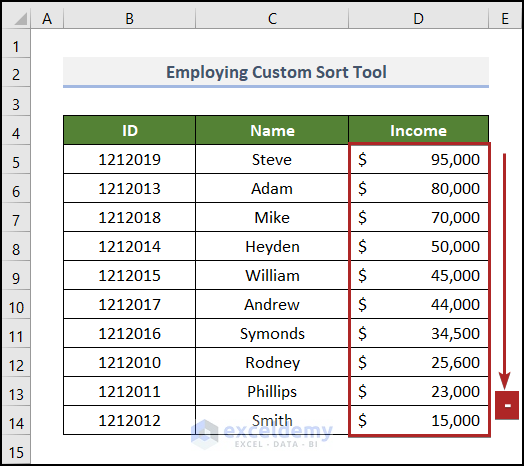
• We can see the column sorted from smallest to largest in our worksheet.

• You can also sort from largest to smallest in a similar way.

Read More: Excel Sort by Column Without Header

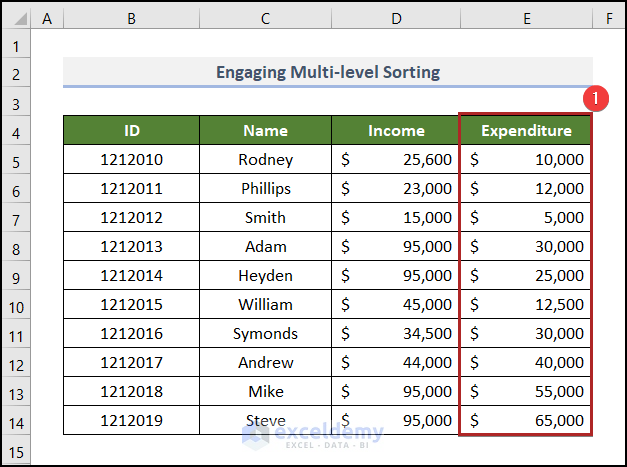
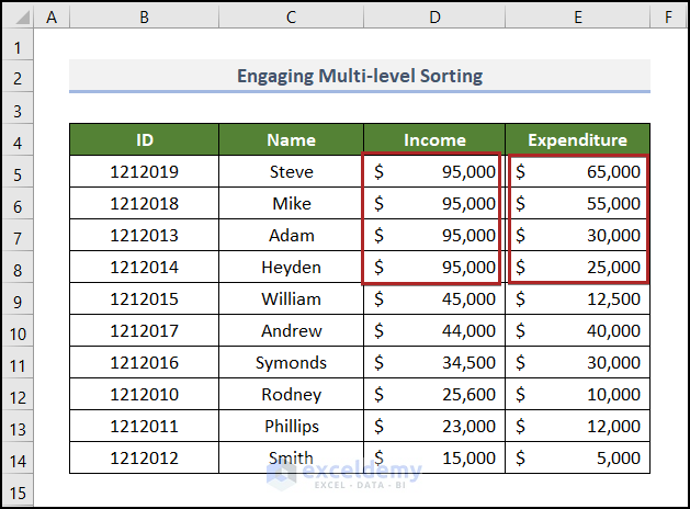
Method 4 – Engaging Multi-level Sorting by Value

We added a new column titled Expenditure and we have changed the income of Mike, Adam, and Hayden to $95,000.

Steps:

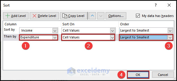
• Open the Sort dialog box.
• Select the sorting style like the previous method.
• Click on Add Level.

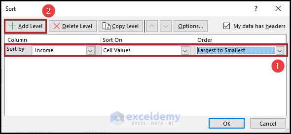
• We will customize this level by the Expenditure column, using the Sort on Cell Values and the Order is Largest to Smallest.
• Click OK.

• We can see that four people have the same top Income, but their Expenditures are also sorted from largest to smallest order.

Method 5 – Inserting the SORT Function

Steps:

• Copy all the column headers and paste them in the F5:H5 range.

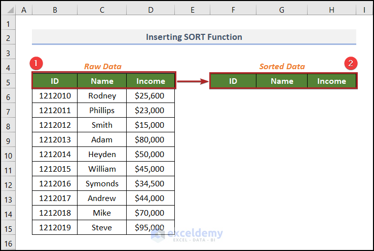
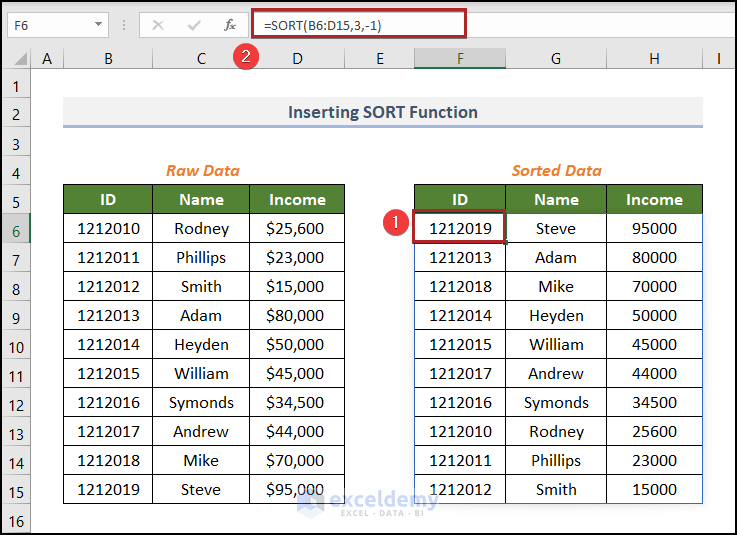
• Select cell F6 and enter the following formula into the Formula Bar.

• Press Enter.

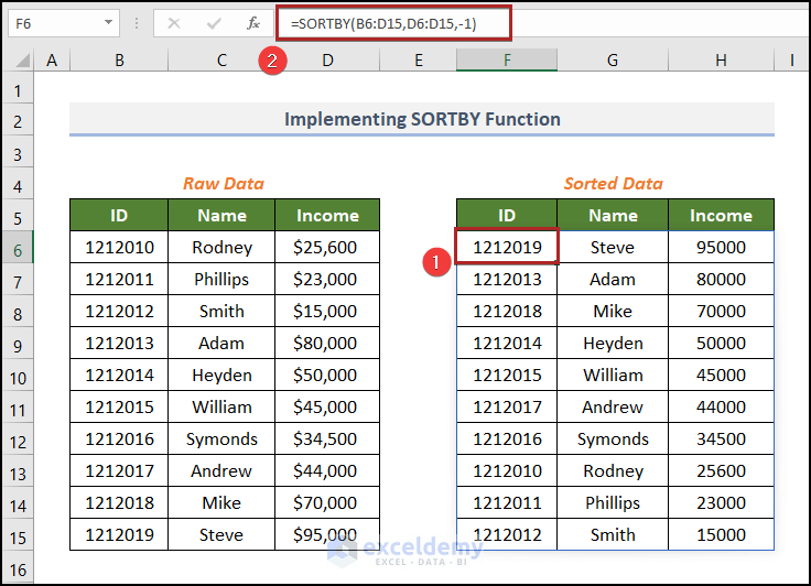
Method 6 – Implementing the SORTBY Function

Steps:

• Select cell F6 and insert the following formula.

• Press Enter.

Read More: Sorting Columns in Excel While Keeping Rows Together

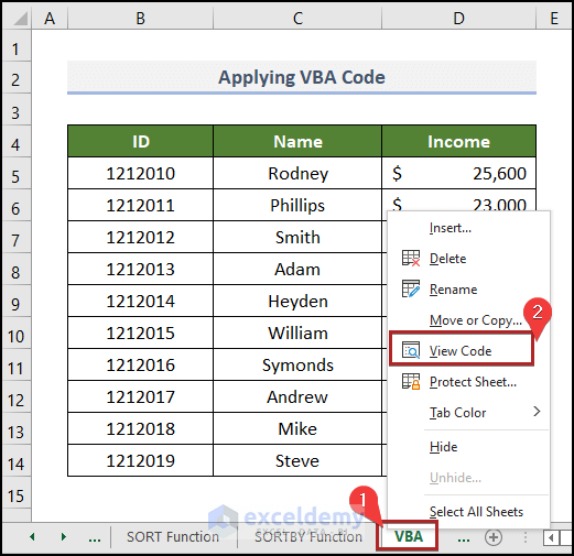
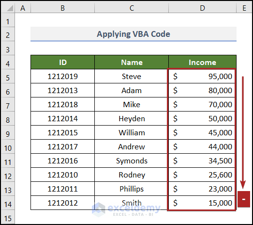
Method 7 – Applying VBA Code

Steps:

• Right-click on the worksheet name.
• From the context menu, select the View Code option.

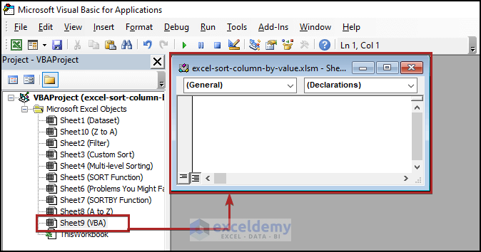
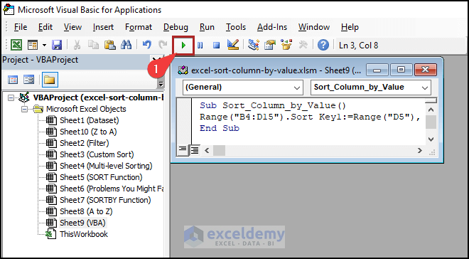
• The Microsoft Visual Basic for Applications window appears. A code module is inserted for Sheet9 (VBA).

• Paste the following code into the module.

Sub Sort_Column_by_Value()
Range("B4:D15").Sort Key1:=Range("D5"), Order1:=xlDescending
End Sub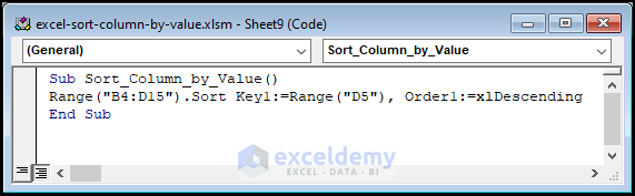

• Run the code.

• The column is sorted from largest to smallest by value.

Read More: How to Sort Columns in Excel Without Mixing Data

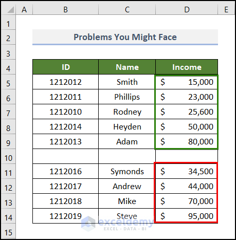
Problems You Might Face While Sorting Column by Value

Though sorting columns by value in Excel is quite easy, you might face some problems if you have Blank or Hidden cells or rows in your data range. See the screenshot below.

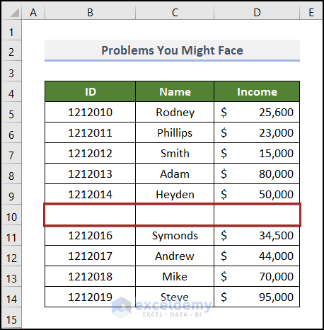
Let’s see what happens when we sort the columns by values.

Only a portion of our data until the first blank cell is sorted, while the remainder remains unsorted.

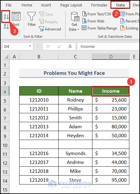
Solution:

• Select all cells in the D4:D14 range instead of just selecting cell D4.
• Go to the Data tab.
• Click on the Sort A to Z icon.

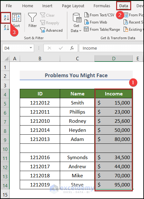
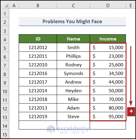
• Excel is showing the correct result.

Things to Remember

➤ The SORT and SORTBY functions are only available for Excel 365. You won’t be able to use this function unless you have this version of Excel.

➤ If you have a blank cell in your data table, select the whole data table to sort by value.

➤ You can auto-sort columns by their value when you use the SORT function.

➤ Always select the column header cell when you sort your data.

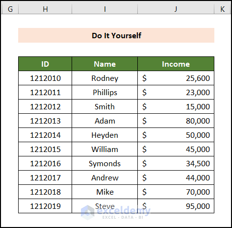
Practice Section

We have provided a Practice section like the one below on each sheet on the right side.

Download the Practice Workbook

<< Go Back to Sort in Excel | Learn Excel