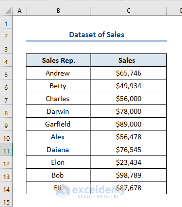
How to Auto Sort Multiple Columns in Excel (2 Useful Methods)

We have made a dataset named Dataset of Sales. It has column headers Sales Rep. and Sales.

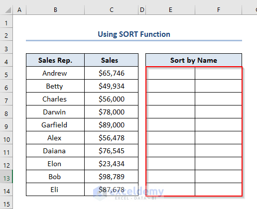
Method 1 – the Using SORT Function

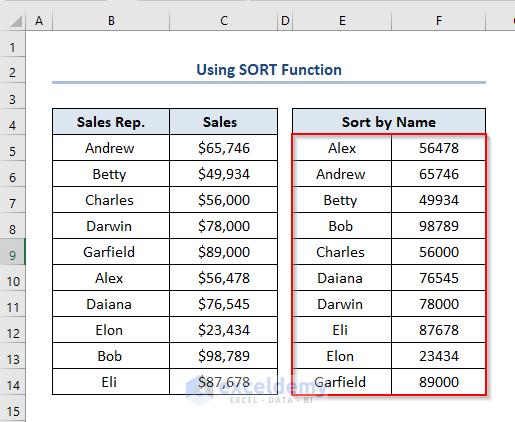
We need to sort Sales Rep. alphabetically in Column E and the sorting of Sales will also change according to the change of Sales Rep.

Steps:

Use the SORT function.
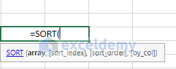
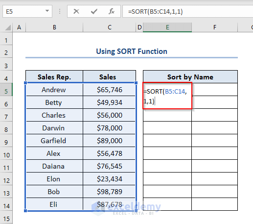
Insert the formula in the E5 cell like this.

=SORT(B5:C15,1,1)

“Array” is our data range (B5:C15). B5:C15 refers to the cell range of Sales Rep. and their corresponding Sales. [sort_index] is the column we want to sort on (1). [sort_order] is where we can specify whether to arrange in ascending or descending order.

Press Enter.

Note: As we are using Microsoft 365, we have got all the outputs from E5:F15 by only inserting the formula in the E5 cell. If you use another version of Microsoft, you may need to use the Fill Handle to get all the outputs.

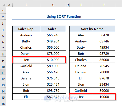
If we change a name in the B9 cell, it will be sorted.

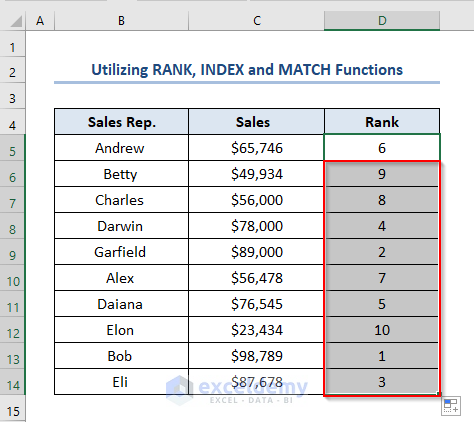
Method 2 – Utilizing RANK, INDEX, and MATCH Functions

Steps:

Use the following formula in the D5 cell.

=RANK(C5,$C$5:$C$14)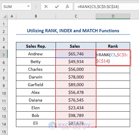

Press Enter.
Use the Fill Handle by dragging down the cursor while holding the bottom-right corner of the D5

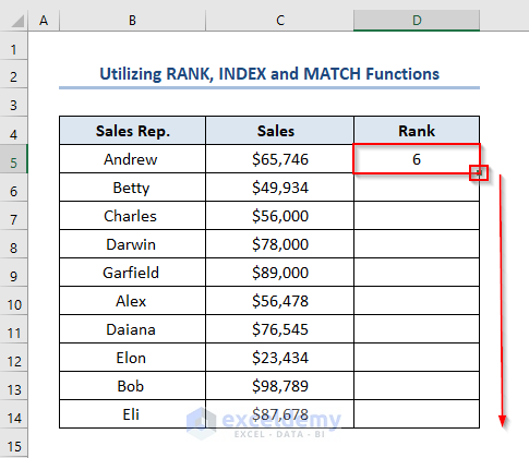
In the Rank column, the ranks will be added for different Sales Rep. as outputs.

We will auto-sort this Rank and Sales Rep.

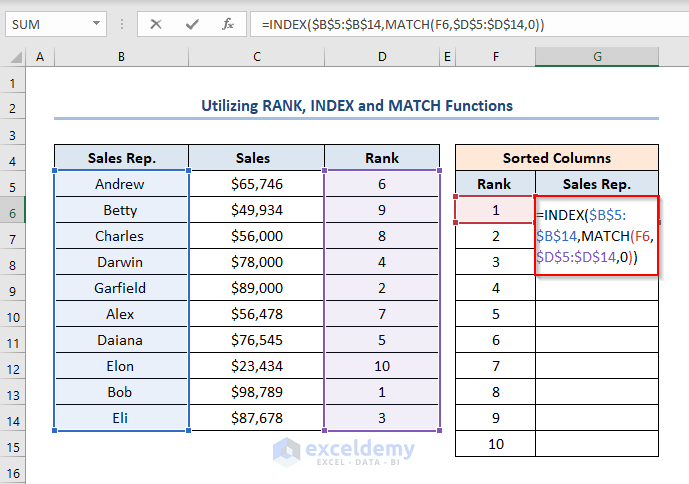
Create another table, and in the “Rank” column, input 1 to 10 serially.

Use INDEX and MATCH functions to sort the ranks.

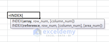
Insert this formula in the G6 cell:

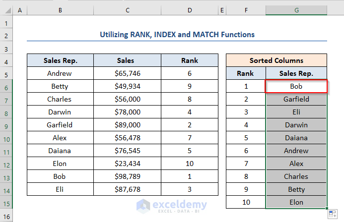
=INDEX($B$5:$B$14,MATCH(F6,$D$5:$D$14,0))

“Array” is the range of cells from where we want to return a value (B5:B14). Block it by pressing F4. To pick the row number, use the “MATCH” function within the “INDEX” function. For “lookup_value” select the Rank number (F6). For “lookup_array” select the array (D5:D14). Block it by pressing the F4 key. We selected “Exact match”.

Press Enter and use the Fill Handle.

Read More: How to Auto Sort Table in Excel

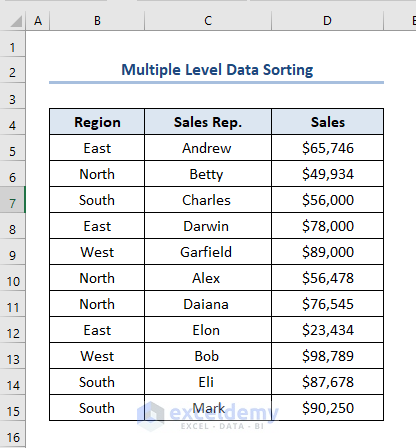
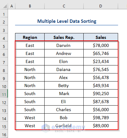
How to Do Multiple Level Data Sorting in Excel

We have the following dataset with column headers as Region, Sales Rep., and Sales. We need to sort the Region column by A to Z and then sort Sales from Largest to Smallest.

Steps:

Select the cells B4:D15.
Go to Data and choose Sort.

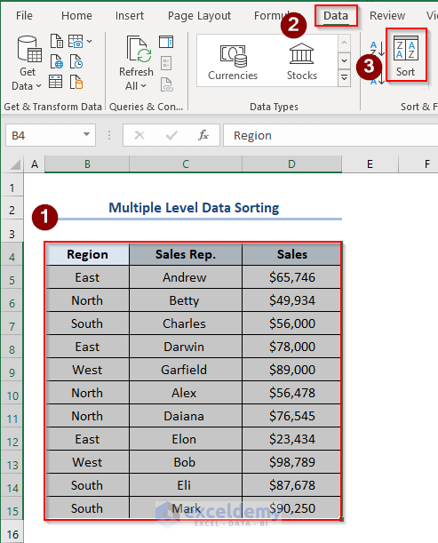
A Sort window will appear like this.
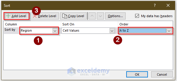
Select Region in the Sort by box as we want to sort based on Region Then choose A to Z in the Order box.
Click Add Level.

Select Sales in the Then by box and choose Largest to Smallest in the Order box.
Click OK.

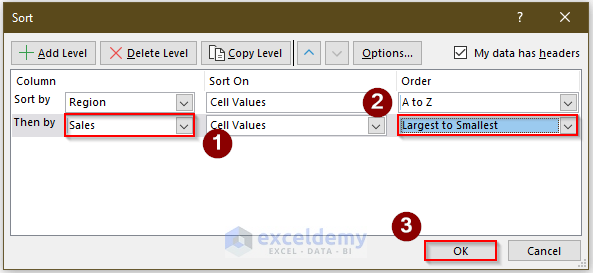
The Region column is sorted according to A to Z order first and then the Sales column of individual sales is sorted according to Largest to Smallest.