In this article, we’ll demonstrate how to use the SORT function or combine it with other functions to sort data automatically when data is changed later.
Example 1 – Auto Sort in Descending Order When Data Changes
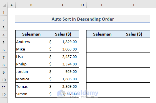
In the following dataset, there are sales values of some salesmen in the first table. In the second table, we’ll use the SORT function to sort the first table by those sales values in descending order, and then change a sales value to see if the table auto sorts.
The generic formula of the SORT function is:
=SORT(sort_array, [sort_index], [sort_order], [by_col])
Steps:
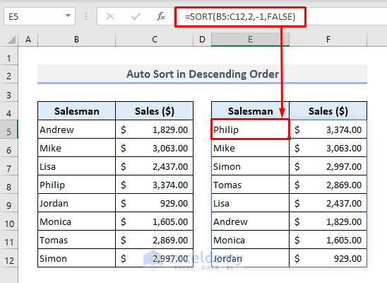
- In the output Cell E5 enter the following formula:
=SORT(B5:C12,2,-1,FALSE)- Press Enter .
The function will return a sorted array with the sales values in descending order.
- Change any of the sales data in the first table, for example in Cell C9 type 4000.
- Press Enter.
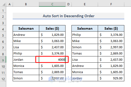
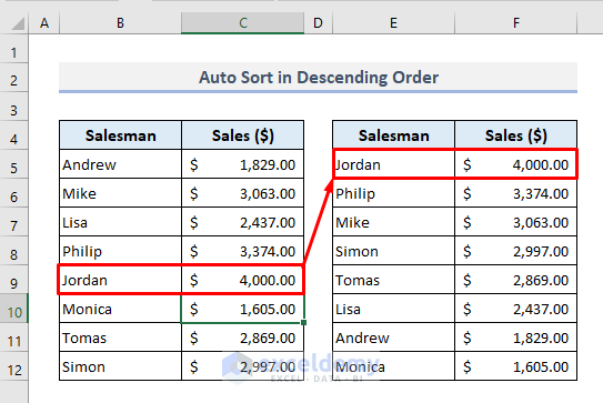
The sales value of Jordan is in a new row based on the position of the sales value.
Read More: How to Auto Sort Multiple Columns in Excel
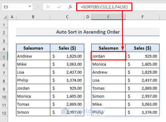
Example 2 – Auto Sort in Ascending Order When Data Changes
To sort the given table in ascending order, simply change the third argument ([sort_order]) to ‘1’ (which denotes ascending order) in the previous formula.
The required formula in Cell E5 is now:
=SORT(B5:C12,2,1,FALSE)After pressing Enter, the entire table data is sorted by sales values in ascending order.
Change any sales value in Column C, and the sorted table will rearrange itself accordingly.
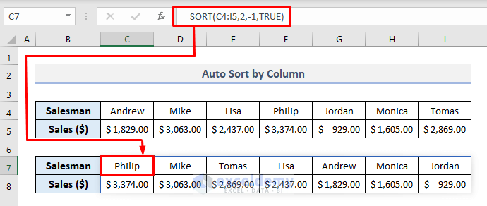
Example 3 – Auto Sort by Column When Data Changes in Excel
Let’s transpose all data in the previous table, so that the columns are converted into rows. We’ll need to sort the table data by the columns in Row 5, where the sales data are situated after being transposed.
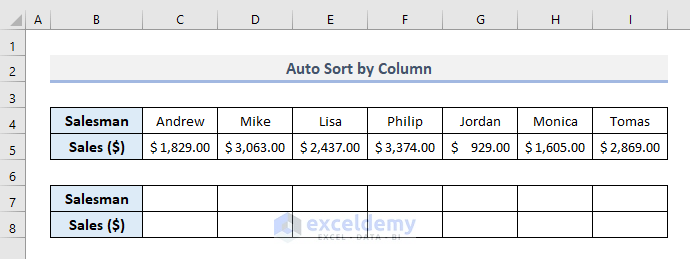
The required formula to sort the table by columns in Cell C7 is:
=SORT(C4:I5,2,-1,TRUE)Press Enter and the sales data will be in descending order in Row 8.
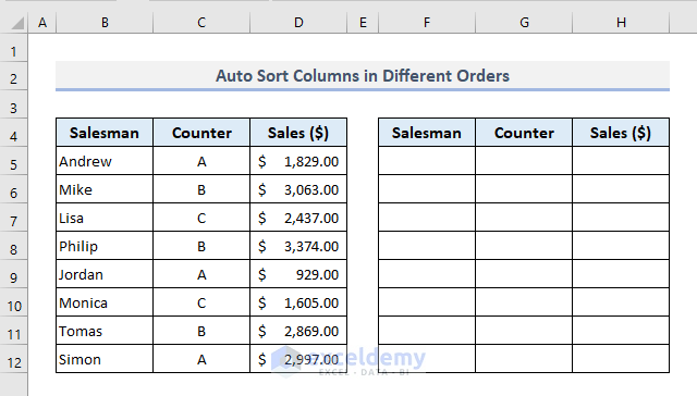
Example 4 – Auto Sort Columns by Different Orders When Data Changes
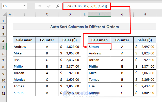
In the modified dataset below, add a new column with the header Counter. We’ll now consider both the Counter and Sales columns, and sort the entire table data using the criteria of ascending and descending orders in the Counter and Sales columns respectively.
For example, after sorting, the letter ‘A’ will be shown three times in a row at the top of the Counter column, and the corresponding sales values will be sorted in descending order.
In the output Cell F5, the required formula is:
=SORT(B5:D12,{2,3},{1,-1})Press Enter and the sorted table will appear. Change any sales data in Column D, and the sorted table will automatically update.
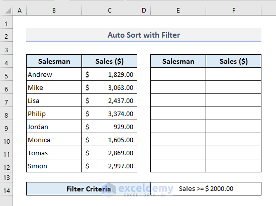
Example 5 – Auto Sort by Filtering When Data Changes in Excel
The FILTER function simply filters a range or an array based on the given conditions or criteria. By using the FILTER function inside the SORT function, we can extract a range of rows from the primary table based on the given condition(s) and then sort them in a specified order.
For example, from the following dataset, we’ll filter the rows for sales values greater than or equal to $ 2000, then use the SORT function to sort those extracted rows in descending order.
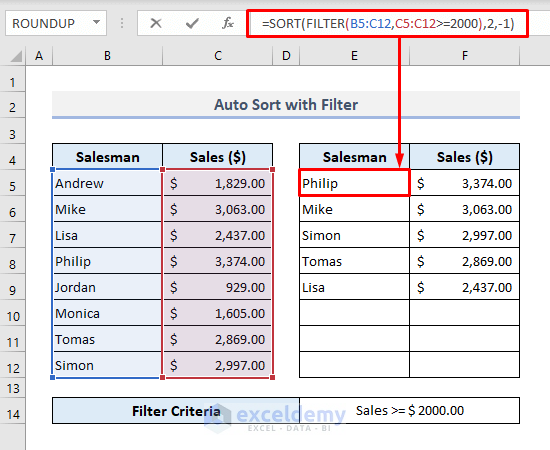
The required formula in the output Cell E5 is:
=SORT(FILTER(B5:C12,C5:C12>=2000),2,-1)Press Enter and the final output with the given conditions is as shown in the picture below. Alter any data in the Sales column in the first table to see the changes in the sorted table.
Read More: How to Auto Sort in Excel When Data Is Entered
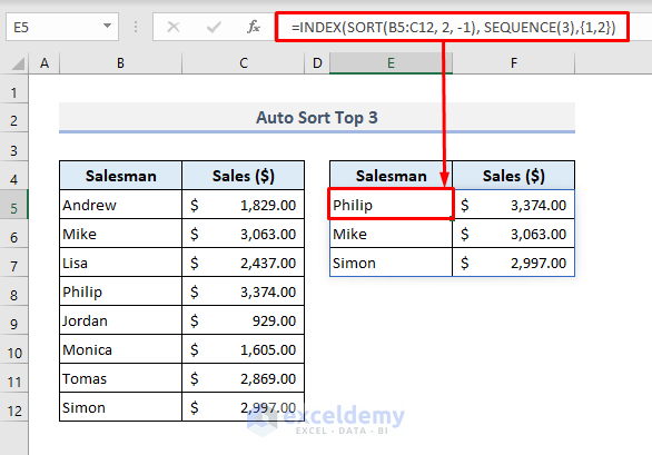
Example 6 – Auto Sort Top 3 When Data Changes in Excel
By combining the INDEX, SORT, and SEQUENCE functions, we can extract three (or any number of) rows containing the top sales values, then sort them in descending order.
The required formula in the output Cell E5 is:
=INDEX(SORT(B5:C12, 2, -1), SEQUENCE(3),{1,2})After pressing Enter, the top 3 sales values in descending order appear in the new table.
How Does the Formula Work?
- The SORT function inside the INDEX function defines the array to sort.
- The SEQUENCE function defines the number of rows that will be extracted from the array.
- In the third argument ([column_num]) of the INDEX function, the index numbers of both columns have been assigned to obtain output with those two columns from the primary table.
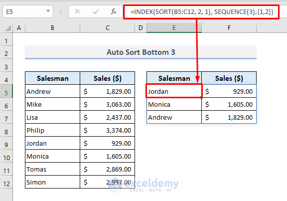
Example 7 – Auto Sort Bottom 3 When Data Changes in Excel
To get the bottom or lowest three sales values, only a minor change in the previous formula is required. As we have to extract the sales values in ascending order, the third argument ([sort_order]) of the SORT function will be ‘1’ now.
The formula required in the output Cell E5 is therefore:
=INDEX(SORT(B5:C12, 2, 1), SEQUENCE(3),{1,2})After pressing Enter, the lowest or bottom three sales values appear in ascending order in the output table.
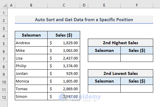
Example 8 – Auto Sort and Get a Value from a Specific Position
By combining the INDEX and SORT functions only, we can extract the second-highest and second-lowest sales values from the table.
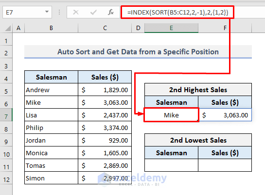
The required formula in Cell E7 is as follows:
=INDEX(SORT(B5:C12,2,-1),2,{1,2})After pressing Enter, the second-highest sales value is returned.
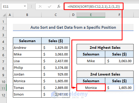
To get the second-lowest sales value, simply change the ‘sort order’ in the SORT function. The required formula in Cell E11 is therefore:
=INDEX(SORT(B5:C12,2,1),2,{1,2})Change any sales data in Column C, and if it matches the criteria of being the second-highest or second-lowest value, the data in the output cells change accordingly.
Example 9 – Auto Sort with Table While Entering New Data
All the methods discussed above are valid for changes to existing data only. But if you append new data to the given table, the sorted array will not change. To automatically update the sorted array to account for new data entries in the primary table, we have to convert the primary table into a filtered table format.
In the following picture, there is no change in the sorted table after the input of new data in the primary table.
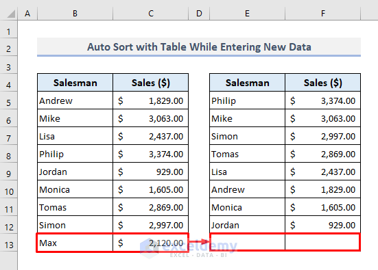
Let’s make the sorted table auto-update after a new input in the primary table.
Steps:
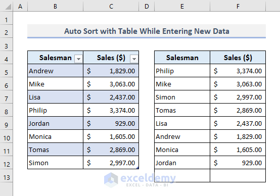
- Select the range of cells of the primary table (B4:C12).
- Press CTRL+T to convert the chart into a filtered table format.
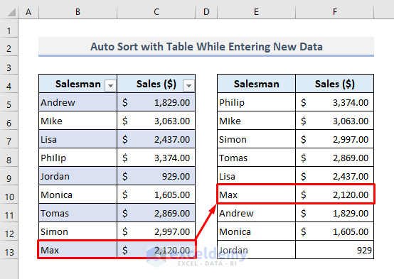
- In Row 13, add new data with the name of a salesman and the corresponding sales value.
The sorted table updates automatically incorporating the new row.
Download Practice Workbook
Related Articles
<< Go Back to Auto Sort in Excel | Sort in Excel | Learn Excel
Get FREE Advanced Excel Exercises with Solutions!
