How to Auto Sort in Excel Without Macros (3 Methods)

This article illustrates 3 methods to auto-sort data in Excel without macros. We’ll use the SORT, VLOOPUP, INDEX, and MATCH functions to sort a specific range of data. Normally when we sort a range of data, it doesn’t update with the changes. We need to apply the sorting feature each time we update a value in the dataset. But it’ll be great if we can make the sorting automatic. Let’s dive into the examples to learn how to make this happen.

How to Auto Sort in Excel Without Macros (3 Easy Methods)

To illustrate the auto sort in Excel, we’re going to use the following dataset. The dataset contains the sale details of different products with their quantity, unit price, and Total Price.

1. Use of SORT Function to Auto Sort in Excel

Introduction to the SORT Function

The SORT function in Excel returns a sorted range of data or array in an ascending or descending order. This function facilitates us in sorting data by one or more columns. It takes several arguments.

=SORT(array, [sort_index], [sort_order], [by_col])
array – range of data or array to sort.
[sort_index] – the column index that is used for sorting. The default value is 1 if omitted.
[sort_order] – use 1 for ascending (default) and -1 for descending order.
[by_col] – to sort data by column use TRUE and use FALSE to sort by row (default).

Task:
We want to auto-sort the dataset according to its quantity (column index=2) in ascending order without macros.

Solution:
To solve the task, we need to configure the arguments like this-
array=range  B5:E13, the whole dataset.
[sort_index]= 2, column 2 holds the quantity values.
[sort_order]=1, sorting is in ascending order.
[by_col]= FALSE, sorting will be in the default way i.e., by row.

Steps:

Follow the steps below.

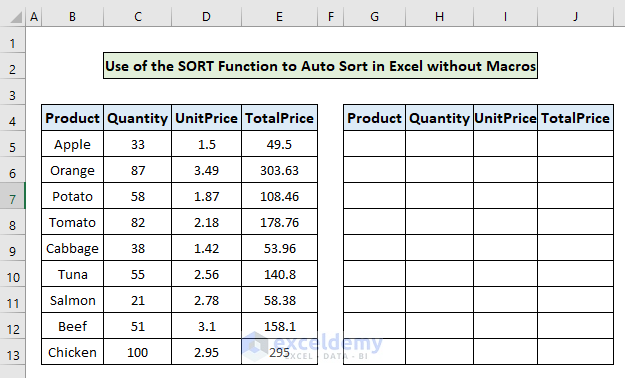
• Create an empty table with the same column header.

• In cell G5, write the following formula.

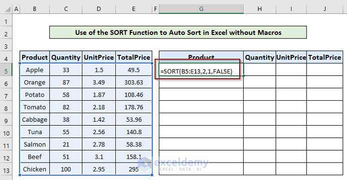
• Now hit Enter to apply the formula.

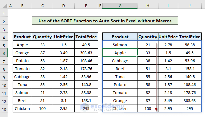
Check the Auto Sort:

Let’s change the quantity of Apple from 33 to 60 in the source table.

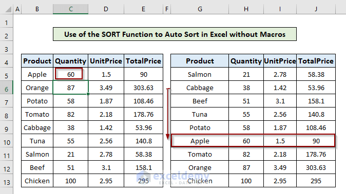
The position of Apple falls from 2nd to 6th in the auto-sorted table.

Read More: How to Auto Sort Multiple Columns in Excel

2. Apply VLOOKUP Function to Auto Sort in Excel

Introduction to the VLOOKUP and RANK Function

The VLOOKUP function in Excel is used to look for data vertically in a table by matching in the first column. The function takes several arguments-

=VLOOKUP(loopup_value, table_array,column_inded_num, [range_lookup])
lookup_value- the value we are looking for that should be in the first column of the table.
table_array– the source data from where we want to retrieve a value.
Column_index_num – the column in the source table from where we want to retrieve a value.
range_lookup– FALSE for an exact match and TRUE for an approximate match.

We also need to use The RANK function before using the VLOOKUP function in this example. The RANK function ranks a number against a given set of numbers from smallest to largest and in reverse as well. The syntax for the function is-

=RANK(number,ref,[order])
number- the number that we want to rank.
ref- the set of numbers to rank against.
[order]- the order is either ascending or descending.

Task:
We want to auto-sort the dataset according to its quantity (column index=2) in ascending order without macros.

Solution:
We need to follow a two-part solution in this example.

Part 1:

We need to rank the quantity of each product against the quantity column itself. For this,

• Create a new column named Rank in the source table.

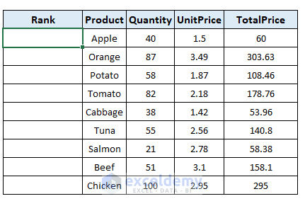
• In cell B5, write down the following formula.

With this formula, we ranked the value 40 at cell D5 in the range $D$5:$D$13 i.e., the Quantity column in the ascending order.

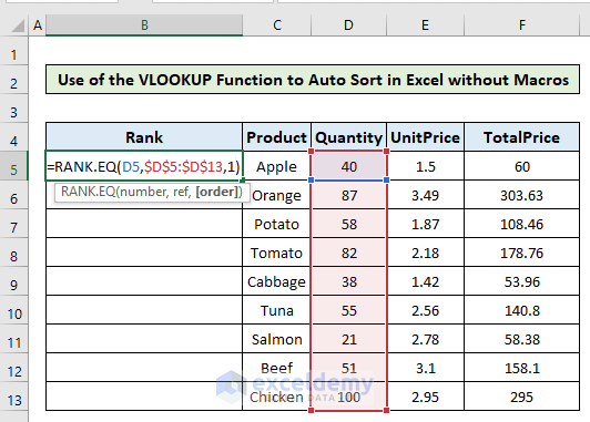
• Hit Enter and then copy the formula to the rest of the column.

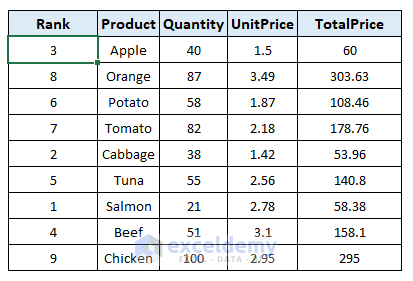
The rank column shows the ranking of each quantity in ascending order.

Part 2:

Now we’ll use The VLOOKUP function to auto-sort the source data. Follow the steps below:

• Create an empty table with the same header as the source table.

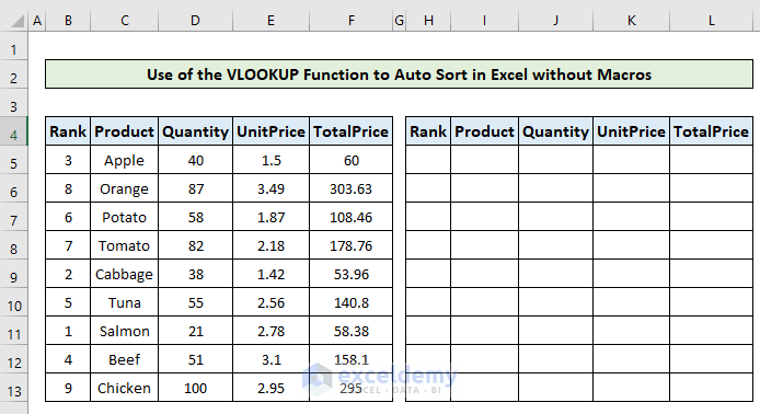
• Write down numbers 1-9 in the Rank column of the new table as we want to auto-sort in ascending order.
• Then in cell I5, put the following formula.

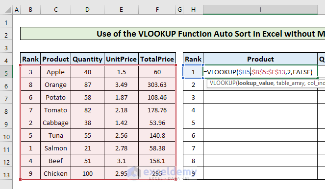
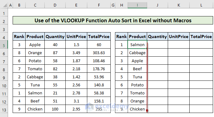
• Press Enter to apply the formula. The first ranked product Salmon is the output.
• Copy the formula to the rest of the column to get the auto-sorted product list.

• Now put the following formula in cell J5 and copy it throughout the column to get the auto-sorted quantity column.

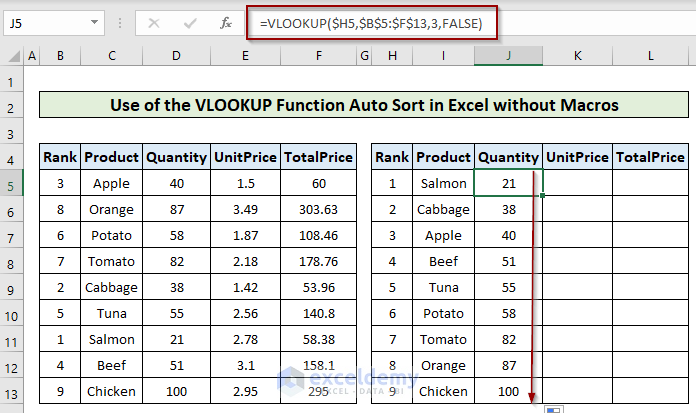
• Use the following formula to get the auto-sorted Unit Price column according to the rank.

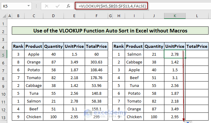
• The total price column is the product of the Quantity and Unit Price columns.

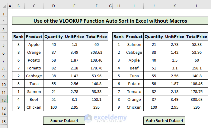
Check the Auto Sort:

Let’s change the quantity of Apple from 40 to 60 in the source table.

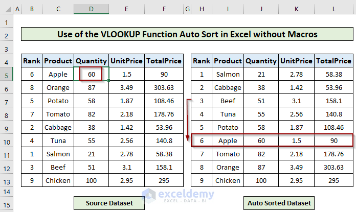
The position of Apple falls from 3rd to 6th in the auto-sorted table.

Read More: Excel Auto Sort when Data Changes

3. Combine INDEX and MATCH Functions to Auto Sort in Excel

The INDEX function is used to find out the value of a specific location in a dataset. In this example,  we used the MATCH function with the INDEX function. The MATCH function provides the location of the cell (row number) that fulfills both of the criteria.

The INDEX function takes the following arguments:

(array, row_num, [col_num])

Now to provide the row number argument of the INDEX function, we used the MATCH function. The MATCH function checks the condition we specified and then outputs the row number of the cell data that fulfills the condition.

The syntax of the MATCH function is-

=MATCH(lookup_value, lookup_array, [match_type])

Task:
We want to auto-sort the dataset according to its quantity (column index=2) in ascending order without macros.

Solution:
Follow part 1 of the previous example to rank the dataset according to the product quantity.

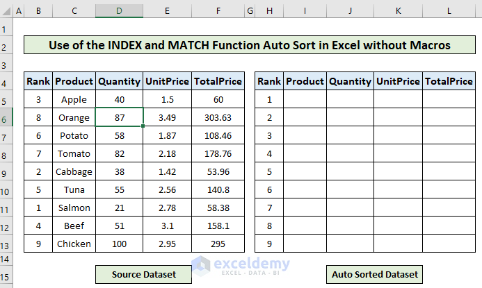
Part 2:

Let’s configure the formula in cell I5. Do the following-

• Write the INDEX function, and select the whole source dataset $B$5:$F$13 as the array argument.

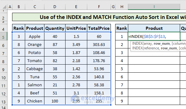
• We supplied the row_num argument of the INDEX function with the MATCH function as

Here,
lookup_value = 1, in cell H5.
lookup_array = $B$5:$B$13, Rank column in the source table.
match_type= 0, for exact match.

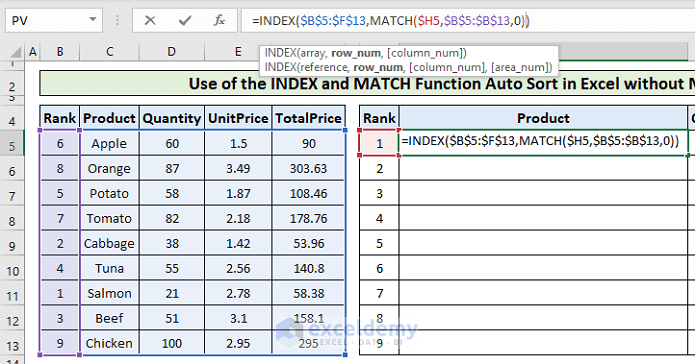
• Finally, we put 2 for the [col_num] argument in the INDEX function as we want to show the product names. The column index 2 in the source dataset represents the product column. So our final formula is-

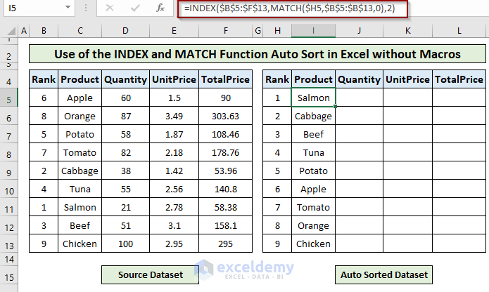
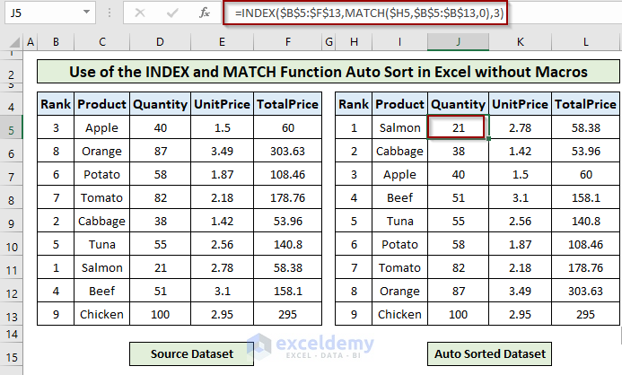
• To get the auto-sorted Quantity and Unit Price column we need to change the [col_num] argument as 3 and 4 respectively in the final formula.

Check the Auto Sort:

Let’s change the quantity of Apple from 40 to 60 in the source table.

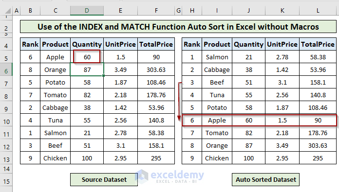
The position of Apple falls from 3rd to 6th in the auto-sorted table.

Things to Remember

• The SORT function is only available in Excel 365.
• We used absolute cell reference for selecting different arguments as they remain the same while copying the formula to other cells.

Download Practice Workbook

Download this practice workbook to exercise while you are reading this article.

Conclusion

Now, we know how to auto-sort in Excel without using macros. Hopefully, it would encourage you to use this more confidently. Any questions or suggestions don’t forget to put them in the comment box below.

Related Articles

• How to Auto Sort Table in Excel
• How to Auto Sort in Excel When Data Is Entered

<< Go Back to Auto Sort in Excel | Sort in Excel | Learn Excel