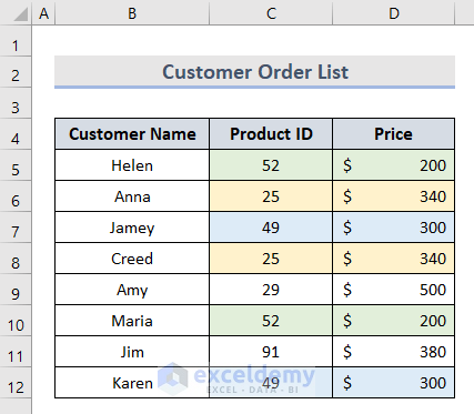
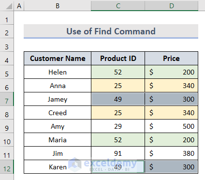
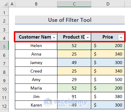
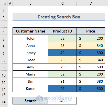
Below is a dataset with information on a company’s Customer Name, Product ID, and Price. We highlighted the cells with similar product ID numbers and price amounts.
Method 1 – Using the Find Command to Select Highlighted Cells
Steps:
- Select cell range C5:D12 as these cells contain highlights.
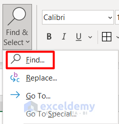
- Go to the Home tab and click the Find & Select drop-down under the Editing group.
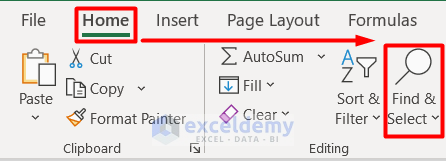
- Select Find from the drop-down menu.
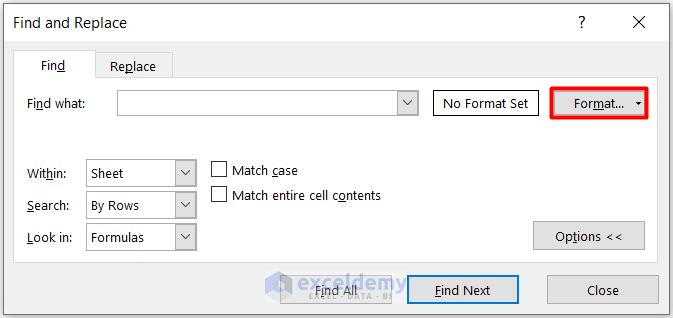
- A new window will appear named Find and Replace.
- Click on Format.
- Select the color from the Background Color palette under the Fill section that you want to find among the highlighted cells.
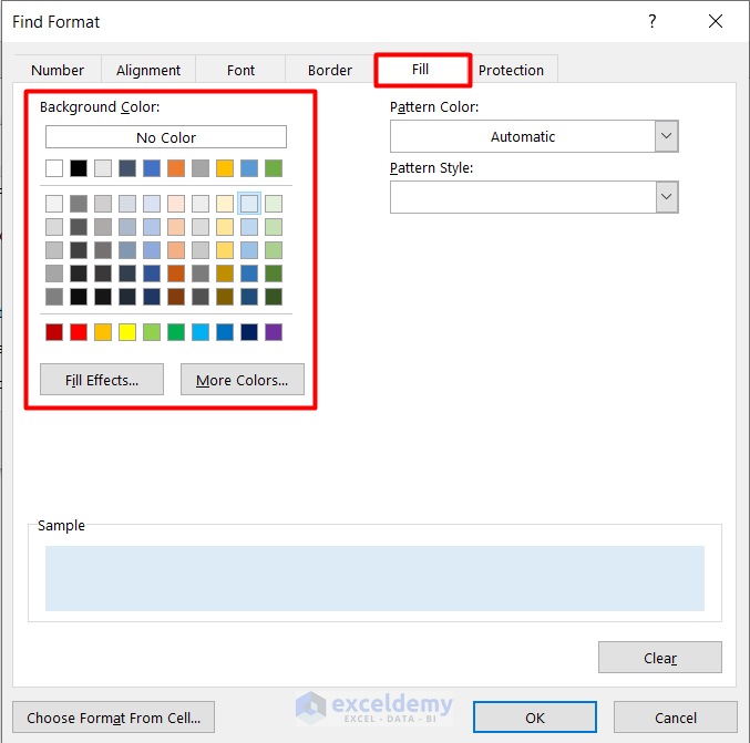
- Press OK.
- Click on Find All.
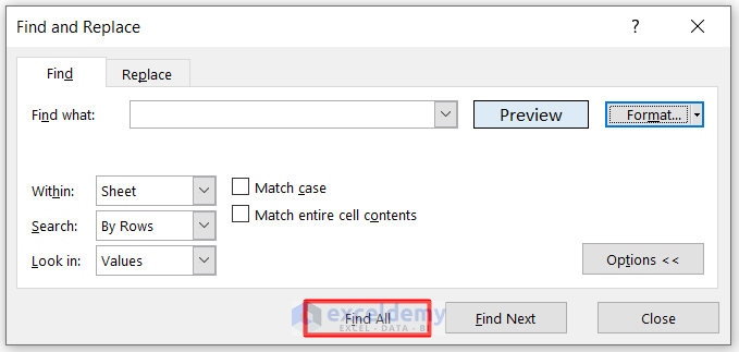
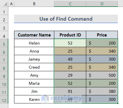
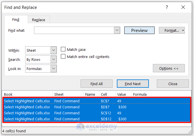
- You will see the list of highlighted cells with the selected color.
- Press Ctrl + A to select all of them.
- Press Close.
- You will see that the specific colored cells are selected.
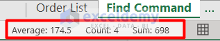
- You can also get the values of the Average, Count, and Sum of the selected cells.
Read More: Select All Cells with Data in Excel
Method 2 – Indicating Highlighted Cells with the Filter Tool
Steps:
- Click on any highlighted cell of your dataset.
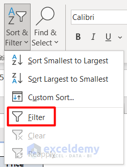
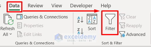
- Go to the Home tab and select Sort & Filter under the Editing group.
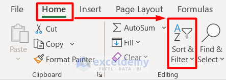
- Select Filter from the drop-down section.
- Or, press Ctrl + Shift + L on your keyboard to get this tool.
- You will see an arrow icon beside each title in the dataset.
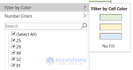
- Click on the arrow beside any of the columns that have highlighted cells. (We selected the Product ID filter icon.)
- Go to Filter by color and choose the color you want to specify.
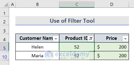
- You will see that only selected colored cells are shown in the worksheet.
Read More: Select All Cells with Data in a Column in Excel
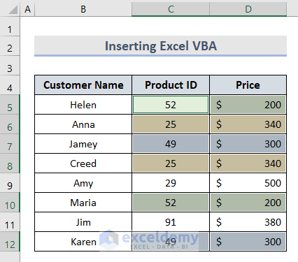
Method 3 – Inserting an Excel VBA Code to Select Highlighted Cells
Steps:
- Sselect cell range B5:D12.
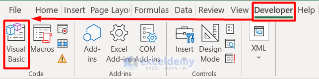
- Go to the Developer tab and select Visual Basic under the Codes group.
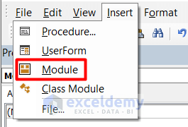
- Select Module under the Insert section in the Visual Basic window.
- Enter the following code on the blank page:
Sub select_highlighted_cells()
Dim rng As Range
Dim selection As Variant
Set rng = Application.selection
mystring = ""
    For Each cellitem In rng
         If cellitem.Interior.ColorIndex <> -4142 Then
            mystring = mystring & cellitem.Address & ","
         End If
    Next
    If mystring = "" Then
        MsgBox "No highlighted cell found"
    Else
        Range(Left(mystring, Len(mystring) - Len(","))).Select
    End If
End Sub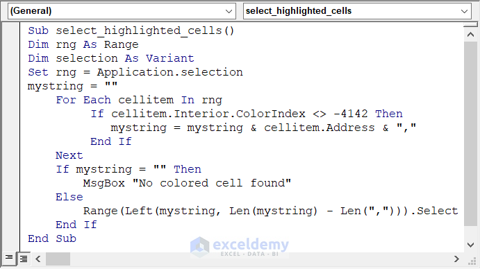
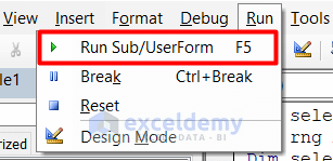
- Click on the Run Sub button or press F5.
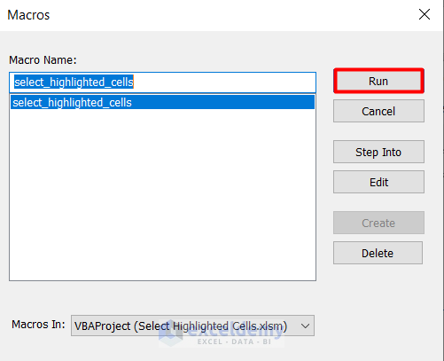
- Select Run on the Macros window.
- You can see that the highlighted cells are selected in the worksheet.
Read More: How to Select Cells with Certain Value in Excel
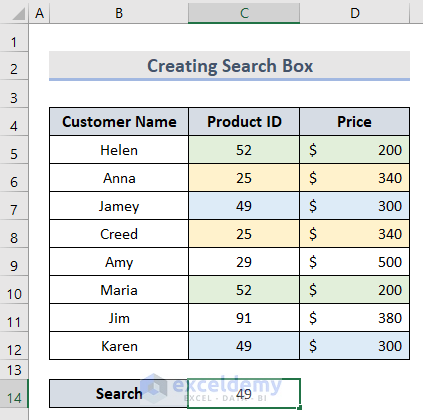
Method 4 – Creating a Search Box in Excel
Steps:
- Create a Search box below the dataset.
- Enter the value you want to find. (We entered the value 49).
- Select cell range B5:D12.
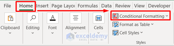
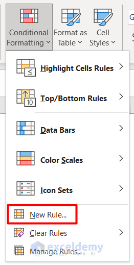
- Go to Home and select Conditional Formatting under the Styles group.
- Select the option New Rule.
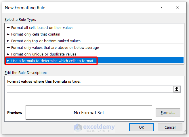
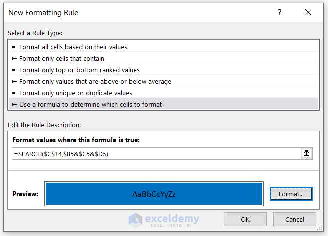
- You will be directed to the New Formatting Rule dialogue box.
- In this window, select the rule like the image below:
- Enter the following formula in the marked box (see screenshot):
=SEARCH($C$14,$B5&$C5&$D5)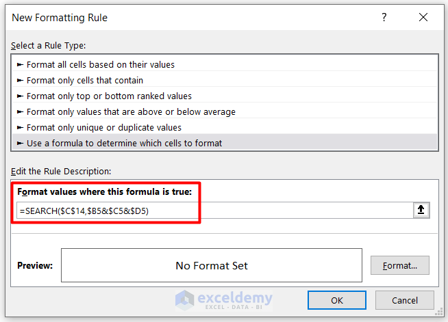
Here, we used the SEARCH function to return the position of a numeric value from one text string and put it inside another cell.
- Click on the Format button.
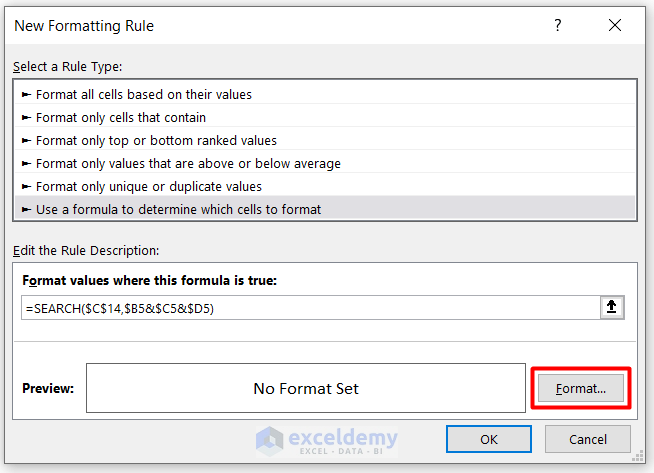
- Select your preferred color from the Background Color palette under the Fill section.
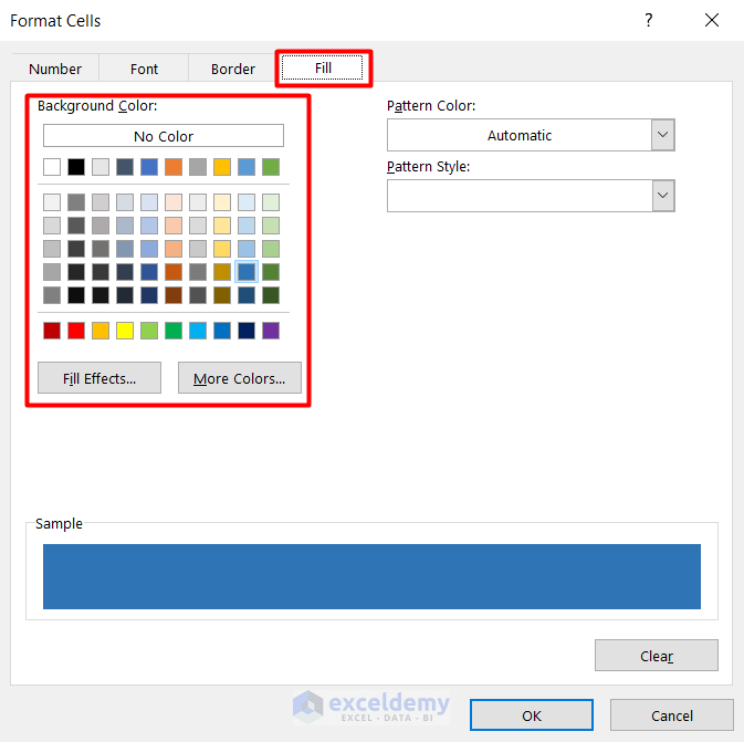
- Press OK.
- Press OK to close the dialogue box.
You will see the searched value is showing with the selected color.
Read More: How to Select Random Cells in Excel
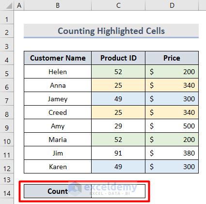
How to Count Highlighted Cells in Excel
Steps:
- Create a Count box like the image below:
- Insert the Filter just like we described in the second method.
- Enter the following formula in cell C14:
=SUBTOTAL(102,D5:D12)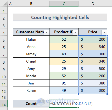
Here, we used the SUBTOTAL function to calculate all the cells. Afterward, put argument number 102 as COUNT. Provided the cell reference as C5:D12.
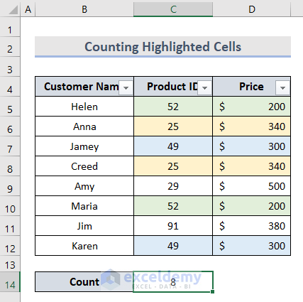
- Press Enter.
You will see the total number of cells on the box.
- Click the filter icon on the Price column.
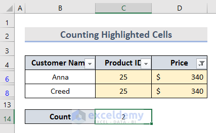
- Apply the Filter by Color tool to select a color.
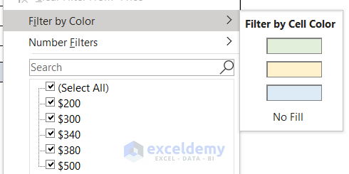
You will see the number of specific colored cells.
Download the Practice Workbook
Download the workbook to practice.
Related Articles
- How to Select Blank Cells in Excel and Delete
- How to Select Only Filtered Cells in Excel Formula
- [Fixed!] Selected Cells Not Highlighted in Excel
- Selecting Non-Adjacent or Non-Contiguous Cells in Excel
<< Go Back to Select Cells | Excel Cells | Learn Excel
Get FREE Advanced Excel Exercises with Solutions!
