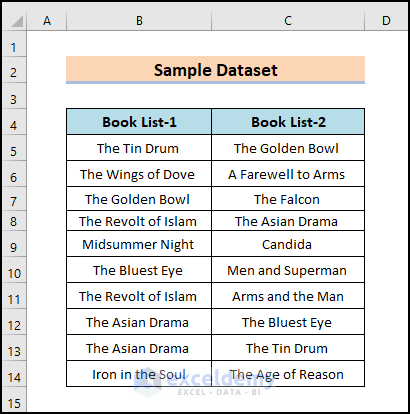
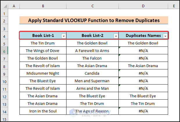
The sample dataset showcases book names in two columns: “Book List-1” and “Book List-2”. To find duplicates and remove them:
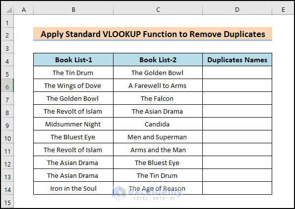
Method 1 – Applying the Standard VLOOKUP Function to Remove Duplicates in Excel
Steps:
- Insert another column: Duplicate Names.
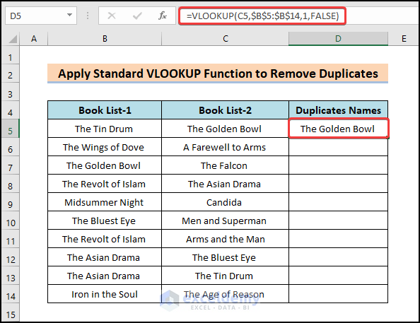
- Select D5 and enter the following formula.
=VLOOKUP(C5,$B$5:$B$14,1,FALSE)
The Lookup_value is C5, the table_array is $B$5:$B$14. Col_index_num is 1 and [range_lookup] is (FALSE) for an exact match.
- Press Enter.
- Golden Bowl is a duplicate value.
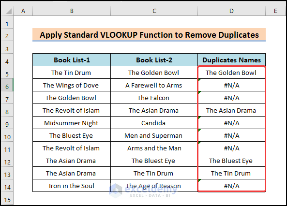
- Drag down the Fill Handle to see the result in the rest of the cells.
- If there are unique values in those two columns, the function will return the #N/A error.
Filter duplicate and unique values:
- Go to the Home tab and select Sort & Filter > Filter.
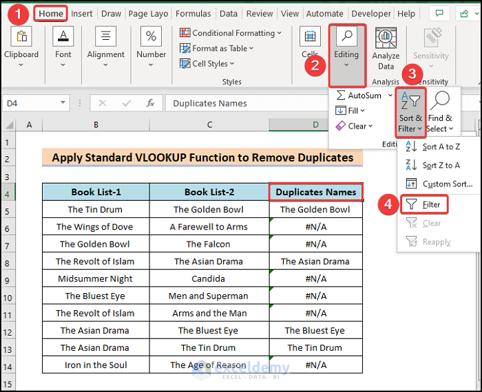
- The Filter icon is displayed in every column.
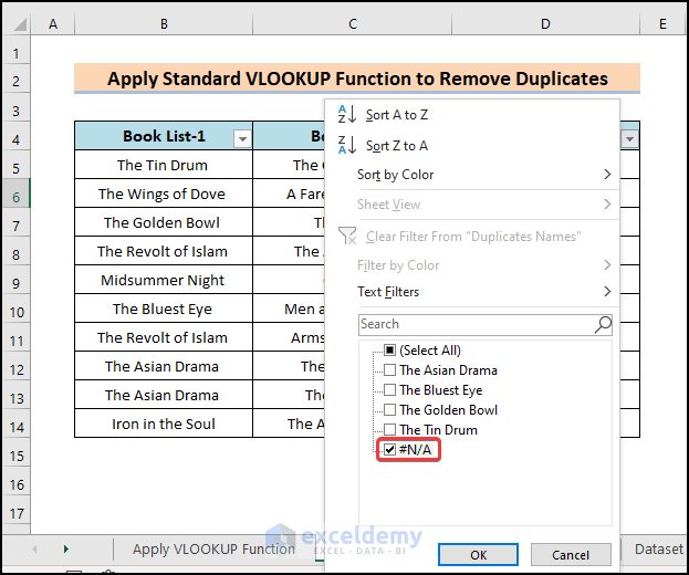
- Click the drop-down icon in Duplicate Values and check #N/A.
- Click OK.
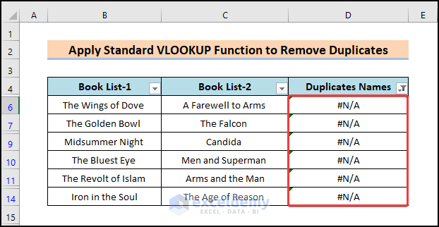
This is the output.
Read More: How to Remove Duplicates Based on Criteria in Excel
2. Combine the VLOOKUP and the ISERROR Functions to Remove Duplicates
2.1 Eliminate Duplicates in the Same Worksheet
Steps:
- Use the same dataset.
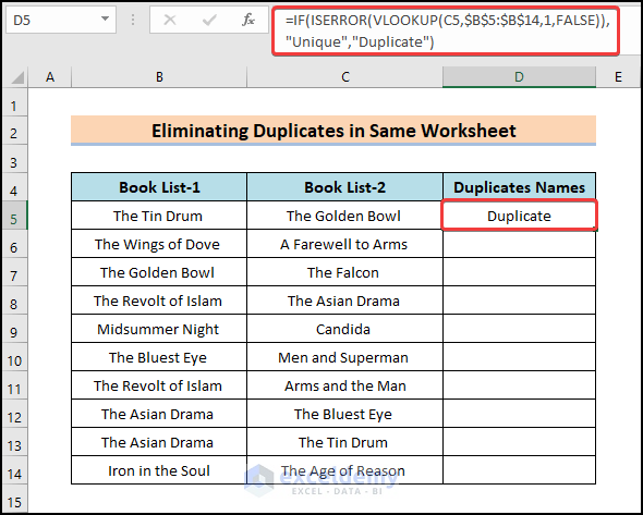
- Enter the formula in D5.
=IF(ISERROR(VLOOKUP(C5,$B$5:$B$14,1,FALSE)),"Unique","Duplicate")
- Press Enter.
- Golden Bowl is a duplicate value.
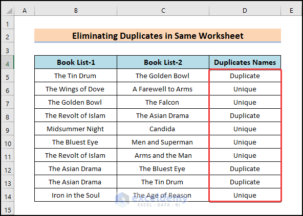
- Drag down the Fill Handle to see the result in the rest of the cells.
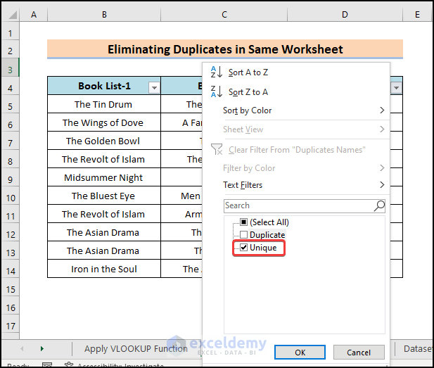
Filter duplicate and unique values:
- Go to the Home tab and select Sort & Filter > Filter.
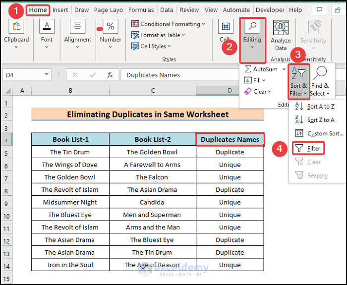
The Filter icon is displayed in every column.
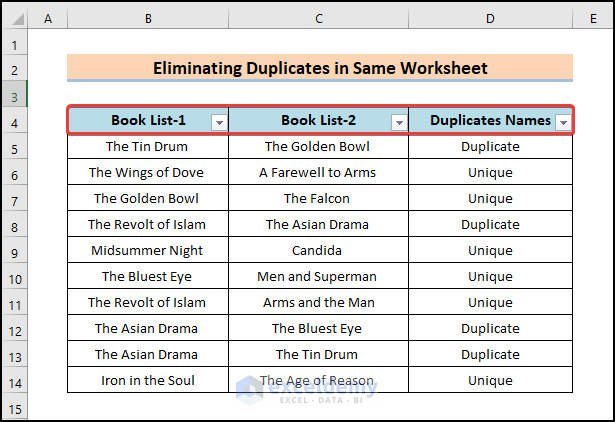
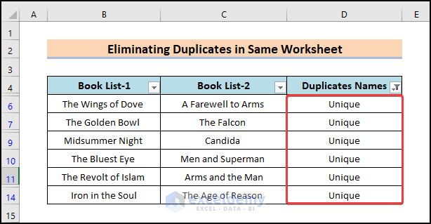
- Check Unique as filtering option and click OK to remove duplicates.
This is the output.
Formula Breakdown
- VLOOKUP(C5,$B$5:$B$14,1,FALSE): finds the exact match of C5 in $B$5:$B$14. The Lookup_value is C5 and the Table_array is $B$5:$B$14. Col_index_num is 1 and [range_lookup] is (FALSE) for an exact match.
- IF(ISERROR(VLOOKUP(C5,$B$5:$B$14,1,FALSE)),”Unique”,”Duplicate”): If the value is true, the formula will return “Unique”. If the value is false, the formula will return “Duplicate’’.
Read More: How to Use Formula to Automatically Remove Duplicates in Excel
2.2 Remove Duplicates in Different Worksheets
Steps:
- Create a dataset in a worksheet.
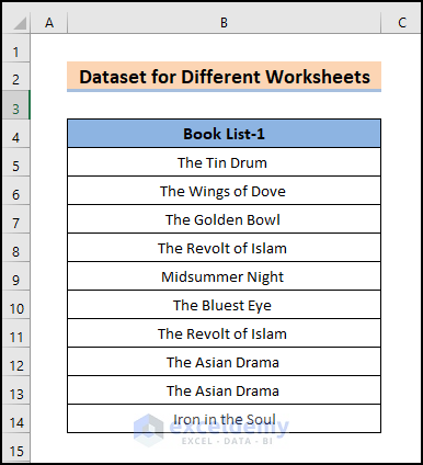
- Create another dataset in another worksheet.
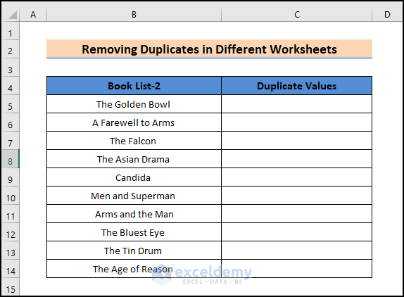
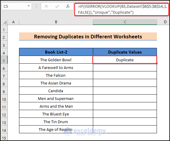
- In C5, enter the formula:
=IF(ISERROR(VLOOKUP(B5,Dataset!$B$5:$B$14,1,FALSE)),"Unique","Duplicate")
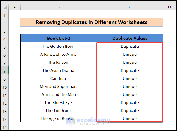
- Press Enter to see the result.
- Drag down the Fill Handle to see the result in the rest of the cells.
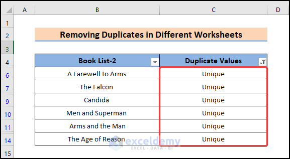
- Remove duplicates using the filter option.
Formula Breakdown
- VLOOKUP(B5,Dataset!$B$5:$B$14,1,FALSE): finds the exact match of C5 in Dataset!$B$5:$B$14. The Lookup_value is B5, the Table_array is Dataset!$B$5:$B$14. Col_index_num is 1 and [range_lookup] is (FALSE) for an exact match.
- IF(ISERROR(VLOOKUP(B5,Dataset!$B$5:$B$14,1,FALSE)),”Unique”,”Duplicate”): If the value is true, the formula will return “Unique”. If the value is false, the formula will return “Duplicate’’.
Read More: How to Find & Remove Duplicate Rows in Excel
2.3 Remove Duplicates in Two Workbooks
Steps:
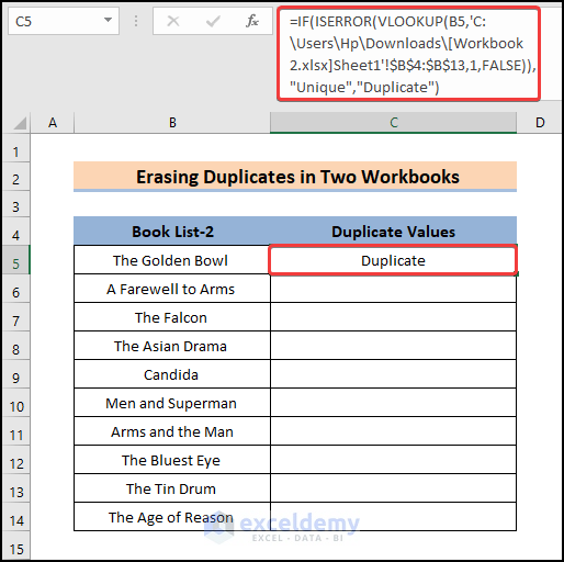
- Enter the formula in C5:
=IF(ISERROR(VLOOKUP(B5,'C:\Users\Hp\Downloads\[Workbook 2.xlsx]Sheet1'!$B$4:$B$13,1,FALSE)),"Unique","Duplicate")
- Press Enter to see the result.
- Drag down the Fill Handle to see the result in the rest of the cells.
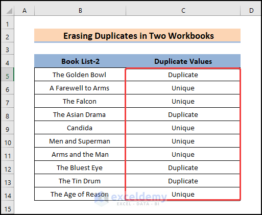
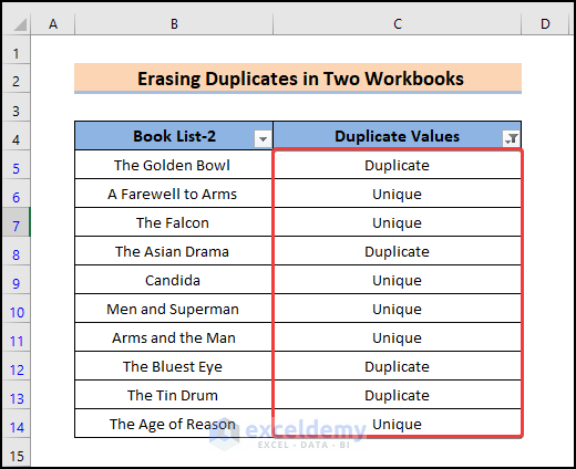
- Remove Duplicate values using the Filter option.
This is the output.
Formula Breakdown
- VLOOKUP(B5,’C:\Users\Hp\Downloads\[Workbook 2.xlsx]Sheet1′!$B$4:$B$13,1,FALSE): finds the exact match of B5 in B4:B13 of sheet 1. The Lookup_value is B5, Col_index_num is 1 and [range_lookup] is (FALSE) for an exact match.
- IF(ISERROR(VLOOKUP(B5,’C:\Users\Hp\Downloads\[Workbook 2.xlsx]Sheet1′!$B$4:$B$13,1,FALSE)),”Unique”,”Duplicate”): If the value is true, the formula will return “Unique”. If the value is false, the formula will return “Duplicate’’.
Things to Remember
- The VLOOKUP function always searches for lookup values from the leftmost top column to the right. This function never searches for the data on the left.
- If you enter a value less than 1 as the column index number, the function will return an error.
- When you select a Table_Array, you have to use an absolute cell reference ($) to block the array.
Download Practice Workbook
Download this practice workbook.
Related Articles
- How to Remove Duplicate Rows in Excel Based on Two Columns
- Hide Duplicate Rows Based on One Column in Excel
- How to Remove Duplicate Rows in Excel Table
<< Go Back to Duplicates in Excel | Learn Excel
Get FREE Advanced Excel Exercises with Solutions!
