Remove Duplicate Rows Except for 1st Occurrence in Excel (7 Ways) -

Method 1 – Remove Duplicate Rows Except 1st Occurrence Using Remove Duplicates Feature

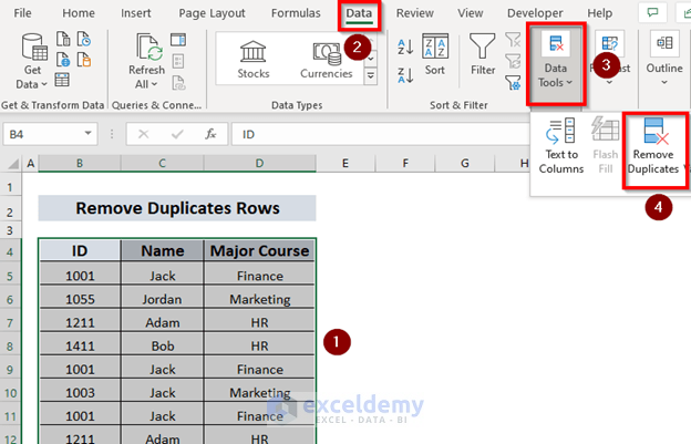
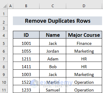
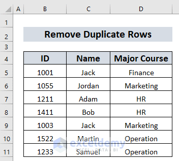
Select the entire datasheet. In the sample dataset, it is B4:D15.
Go to the Data tab >> from Data Tools >> select Remove Duplicates.

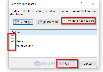
The Remove Duplicates dialog box will open. By default, all the columns are checked and My data has headers box is ticked.

Click OK.

It will remove the duplicate rows.

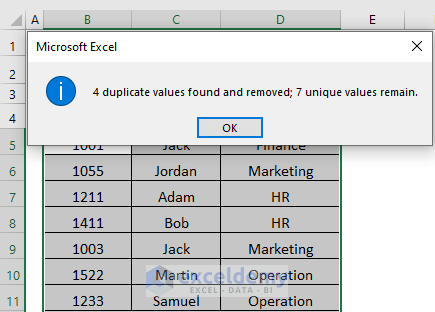
This will be your output.

Method 2 – Remove Duplicate Rows Except 1st Occurrence Using Advanced Filter

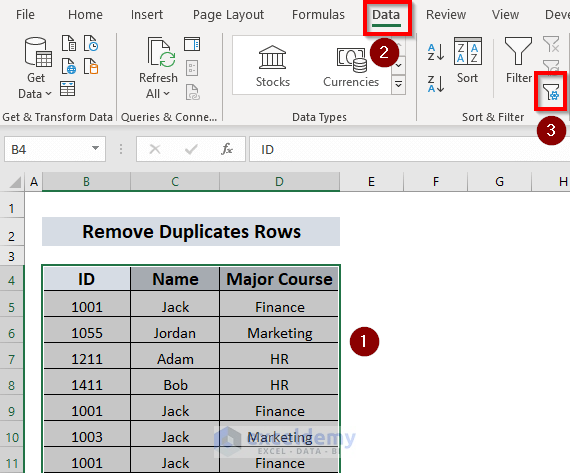
Select the range. In our case it is B4:D15.
Go to the Data tab >> select Advanced Filter.

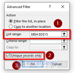
The Advanced Filter window will open.

Enter your range in the List range box and tick the Unique records only box.
Click OK.

The output will be like this.

Method 3 – Remove Duplicate Rows Except 1st Occurrence using UNIQUE Function

Select a cell. In our case it is F4.
Enter the following formula,

=UNIQUE(B4:D15)

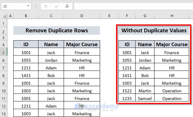
Press ENTER to remove the duplicate values.

After some formatting, this is the output in our worksheet.

Note: The UNIQUE function is available only in the latest versions like Excel 365 and Excel 2021. This method may not work if you are using an older version of Excel.

Method 4 – Remove Duplicate Rows Except 1st Occurrence Using Power Query

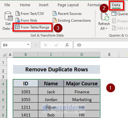
Select the entire data range that you are going to use. In our case it is B4:D15.
Go to Data tab >> select From Table / Range.

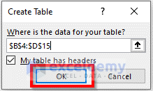
A Create Table window will open.

Click OK.

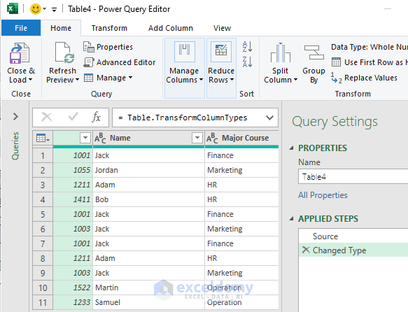
The Power Query window will pop up.

Select the entire table, Right-click on it and select Remove Duplicates.

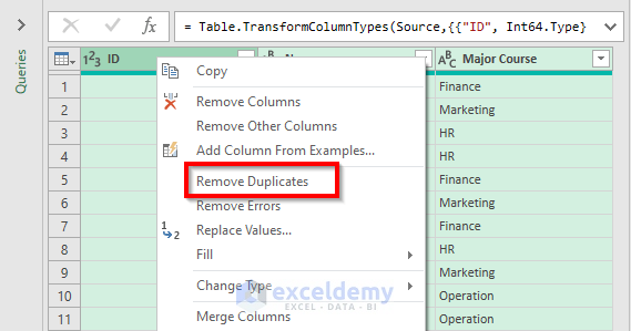
All the duplicate values will be removed.

Transfer this table to your original workbook by clicking Close & Load.

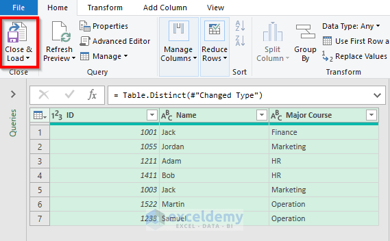
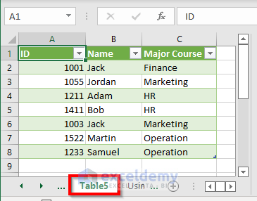
A new sheet will be created in the workbook. Name the table. In our case, it is named as Table5.

Method 5 – Remove Duplicate Rows Except 1st Occurrence Using COUNTIF Function

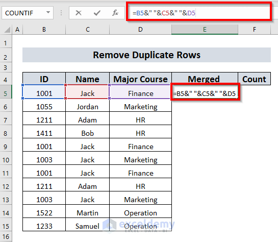
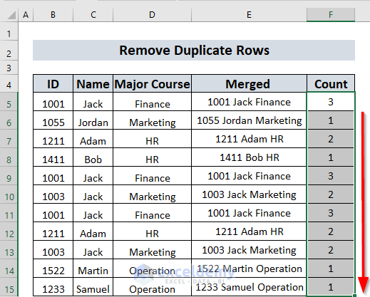
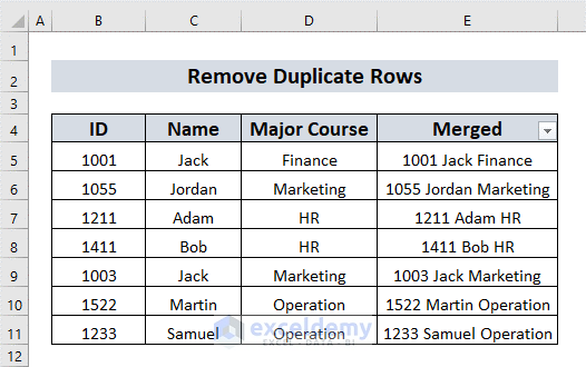
To apply this method, you have to make two new columns in your datasheet. The columns are labeled as Merged and Count.

Enter the formula in cell E5.

=B5&” “&C5&” “&D5

We have used this formula to merge the values of cells B5, C5, and D5. “ ” is used to put a space among these cell values.

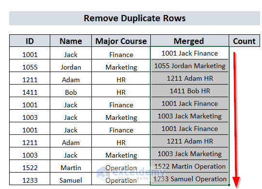
Press ENTER and 1001 Jack Finance will appear in cell E5.

Use the Fill Handle to AutoFill the formula to the remaining cells.

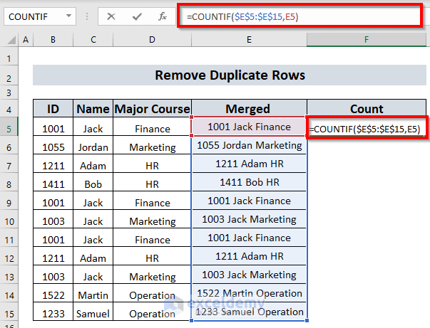
In the F5 cell, enter the following formula,

=COUNTIF($E$5:$E$15,E5)

This formula will tell you how many times a particular cell value appears. For example, when you press ENTER, cell F5 will show 3 in return. This is because the cell value in E5 ( that is, 1001 Jack Finance) is in the range E5:E11 three times (check E5, E9, E11).

Use the Fill handle to AutoFill up to cell F15.

Select the whole dataset, go to Data tab >> select Sort and Filter >> and select Filter.

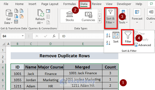
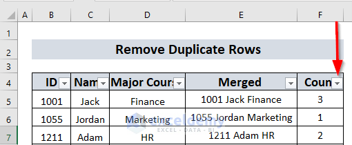
A drop-down menu will appear in each column header.

In the Count column, click the drop-down menu and tick the box for 3.

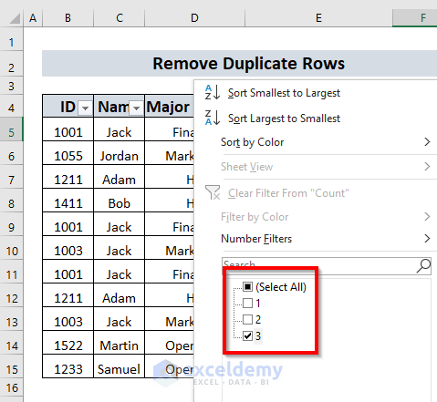
All the rows having 3 in the Count column will show up.

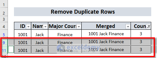
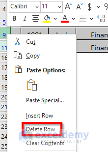
Select all the rows except for the first one, and delete them manually.

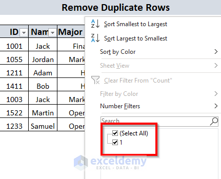
You have to repeat this task for all the boxes until you have only the box containing 1 after clicking the drop down list.

Your result will be as shown below.

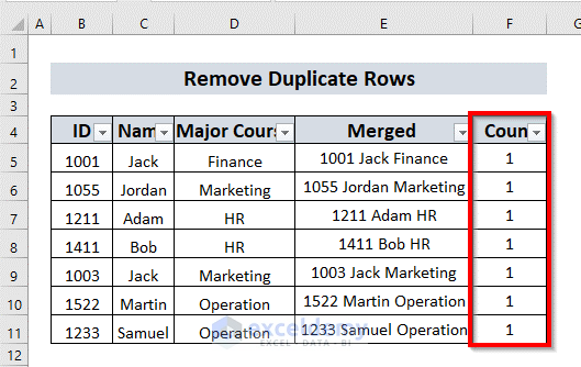
All the duplicate rows have been removed.

Method 6 – Remove Duplicate Rows Except 1st Occurrence Using Conditional Formatting

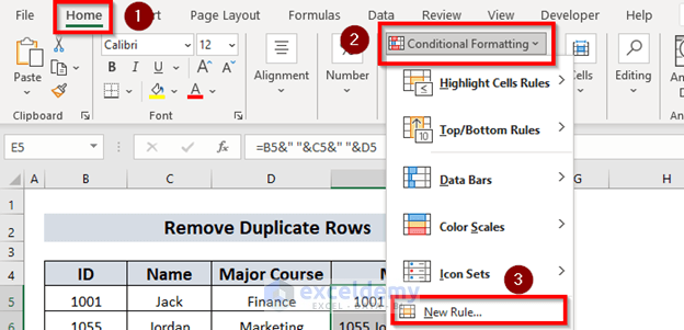
Create a new column. We have named it Merged.
Go to Home tab >> select Conditional Formatting >> select New Rule.

A New Formatting Rule window will open.

Select a Rule Type. In our case, it will be Use a formula to determine which cells to format.
Enter the following formula in the box.

=COUNTIF($E$5:$E5,$E5)>1

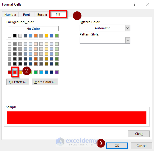
Format as required.

This formula will format the cells that are duplicated in your dataset.

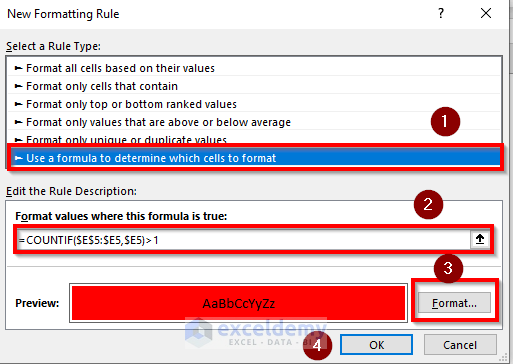
Click OK.

Put Filter on for the Merged column.

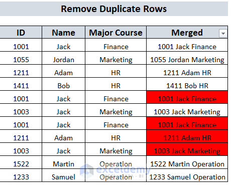
Choose Filter by Color and select the red colored box.

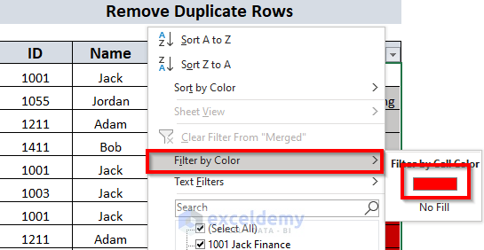
All the red colored cells will open.

Delete the rows using COUNTIF Function.

Method 7 – Remove Duplicate Rows Except 1st Occurrence Using VBA

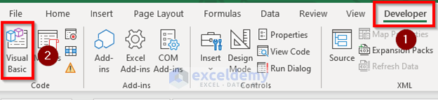
Go to the Developer tab >> select Visual Basic.

Go to Insert tab>>Module.

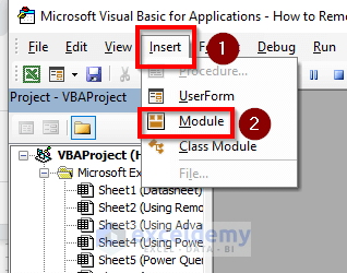
A Module window will appear.

Enter the following code.

Sub RemoveDuplicates ()
Dim Rng As Range
Set Rng = Range("B4:D15")
Rng.RemoveDuplicates Columns:=Array(1, 3), Header:=xlYes
End Sub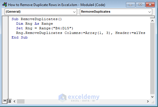

This code will create a macro that will remove duplicate rows from the cell range B4:D15. To do so, we’ve created a Sub Procedure RemoveDuplicates, declared Rng as Range, used the Set method to set the range, and also used the VBA RemoveDuplicates method where in the Array given column numbers 1 & 3 to compare two columns’ values so that it only removes duplicates rows.