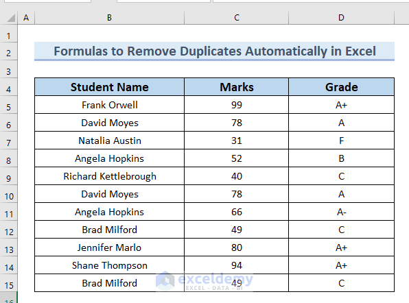
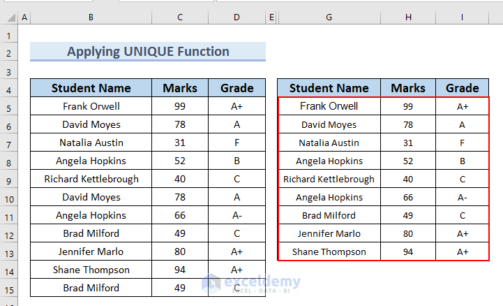
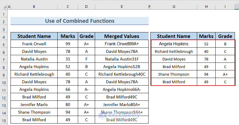
In the following dataset, we have the Student Name, Marks, and Grade columns. The names of some students have been repeated along with their marks and grades. We’ll remove those duplicate rows.
Method 1 – Use the UNIQUE Function to Eliminate Duplicates
The UNIQUE function is only available in Excel 365 onward.
Case 1 – Completely Removing the Values that Appear More than Once
- Use the following formula in cell G5.
=UNIQUE(B5:D15,FALSE, TRUE)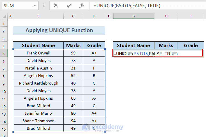
Formula Breakdown
- UNIQUE(B5:D15,FALSE, TRUE) → the UNIQUE function finds a number of unique data in an array.
- B5:D15 → indicates an array.
- FALSE → indicates by_col.
- TRUE → indicates that the duplicates will be removed completely.
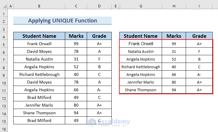
- Hit Enter.
- The unique values will be listed in cells G5:I11.
Notes:
- Three names of the students had duplicates: David Moyes, Angela Hopkins, and Brad Milford.
- Among them, David Moyes and Brad Milford have been removed completely.
- Angela Hopkins has not been removed because the marks and grades of two Angela Hopkins are not the same. That means they are two different students.
Case 2 – Keeping One Copy of the Values that Appear More than Once
- Use the following formula in cell G5.
=UNIQUE(B5:D15,FALSE,FALSE)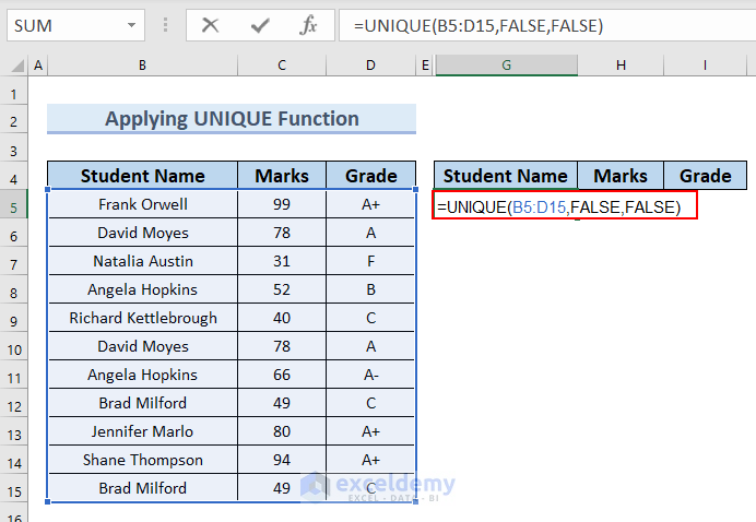
- Hit Enter.
- You can see the result in cells G5:I13.
Read More: How to Remove Duplicates Based on Criteria in Excel
Method 2 – Combine the CONCATENATE, FILTER, and COUNTIF Functions to Remove Clones
Steps:
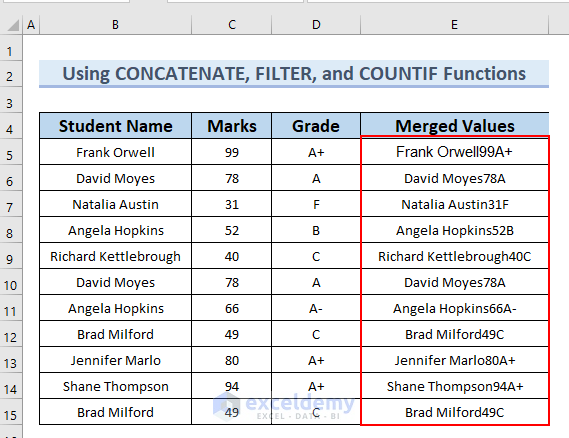
- Make a new column and insert the following formula in cell E5.
=CONCATENATE(B5:B15,C5:C15,D5:D15)The CONCATENATE function sums up three columns into one.
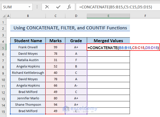
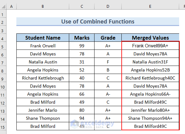
- Press Enter.
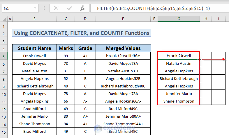
- Go to another new column and insert the following formula in cell G5.
=FILTER(B5:B15,COUNTIF($E$5:$E$15,$E$5:$E$15)=1) 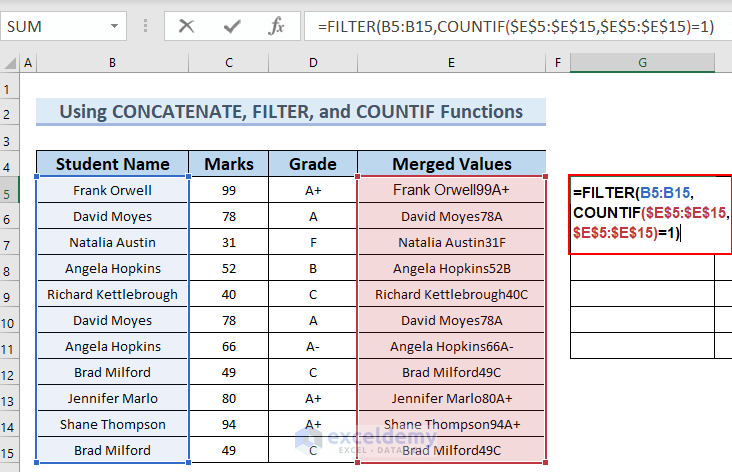
Formula Breakdown
- COUNTIF($E$5:$E$15,$E$5:$E$15)=1 → the COUNTIF function counts cell numbers that meet the criteria.
- FILTER(B5:B15,COUNTIF($E$5:$E$15,$E$5:$E$15)=1) → the FILTER function filters a range of data based on defined criteria.
- Hit Enter.
- You can see the unique values in cells G5:G11.
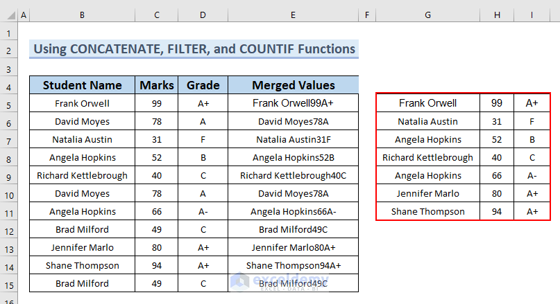
- Drag the Fill Handle right up to the total number of your columns (3 in this example).
- You will get the whole data set without the duplicate values.
Note:
- You can remove all the values that appear more than once.
- You can’t keep one copy of the duplicate values as mentioned in the earlier method.
Method 3 – Merge IFERROR, INDEX, SMALL, CONCATENATE, IF, and COUNTIF Functions
Steps:
- Make a new column and insert this formula in cell E5.
=CONCATENATE(B5:B15,C5:C15,D5:D15) 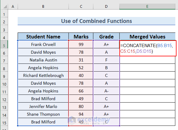
Formula Breakdown
- The CONCATENATE function merges the three columns into one single column.
- Since this is an Array Formula, press Ctrl + Shift + Enter unless you are in Office 365.
- You can see the complete column with merged values.
- Use the following formula in cell G5.
=IFERROR(INDEX(B5:D15,SMALL(IF(COUNTIF(E5:E15,E5:E15)=1,ROW(E5:E15)-ROWS(E2:E4),""),ROW(E5:E15)-ROWS(E2:E4)),{1,2,3}),"")
Formula Breakdown
- The ROWS function finds out the number of rows in an array.
- The IF function does a logical comparison between a given value and the value we expect.
- The COUNTIF function counts a number of cells based on criteria.
- The INDEX function finds the data from a data range.
- The SMALL function gives the output of kth lowest value in an array.
- The IFERROR function returns a blank cell when the formula contains an error.
- Hit Enter.
- The cells G5:I11 do not contain any duplicate values.
Note:
- You can also remove all the values that appear more than once
- However, you can’t keep one copy of the duplicate values as mentioned in the earlier method.
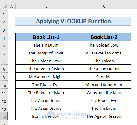
Method 4 – Utilize the VLOOKUP Function for Removing Duplicates Automatically
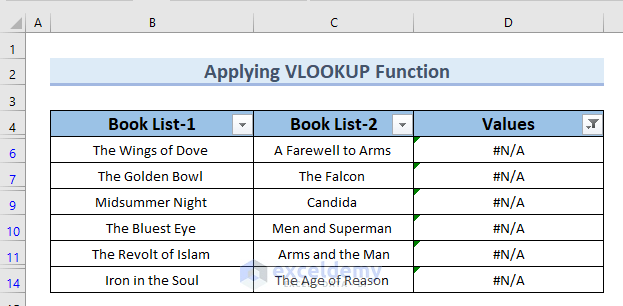
We have modified the dataset to contain the Book List-1 and Book List-2 columns. We will use VLOOKUP to get rid of duplicates.
Steps:
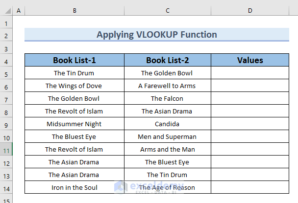
- Create another column D after Book List-2, named Values.
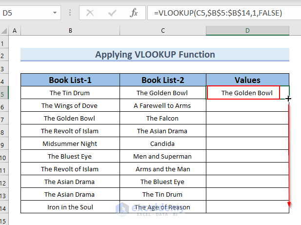
- Select cell D5 and use the following formula.
=VLOOKUP(C5,$B$5:$B$14,1,FALSE) 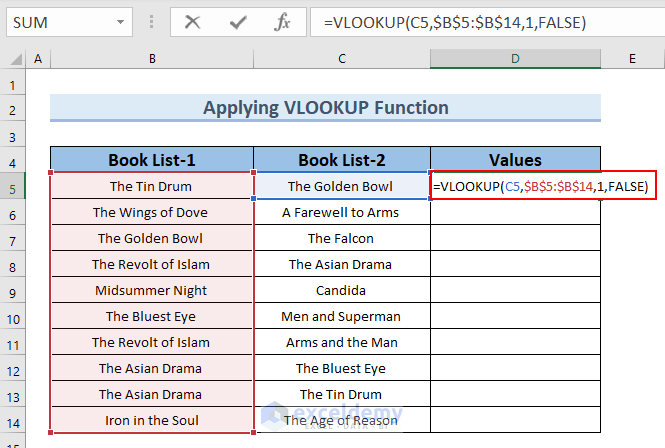
Formula Breakdown
- VLOOKUP(C5,$B$5:$B$14,1,FALSE) → the VLOOKUP function searches for a value in an array.
- Lookup_value is C5.
- Table_array is $B$5:$B$14.
- Col_index_num is 1.
- [range_lookup] is FALSE as we want the exact match
- Output: The Golden Bowl
- Explanation: The Golden Bowl is the duplicate value.
- Hit Enter.
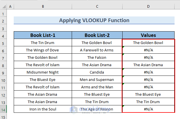
- Drag down the formula with the Fill Handle tool.
- If there are any unique values in those two columns, the function will return the #N/A error.
- Select the headings of the dataset and go to the Data tab.
- From the Sort & Filter group, select Filter.
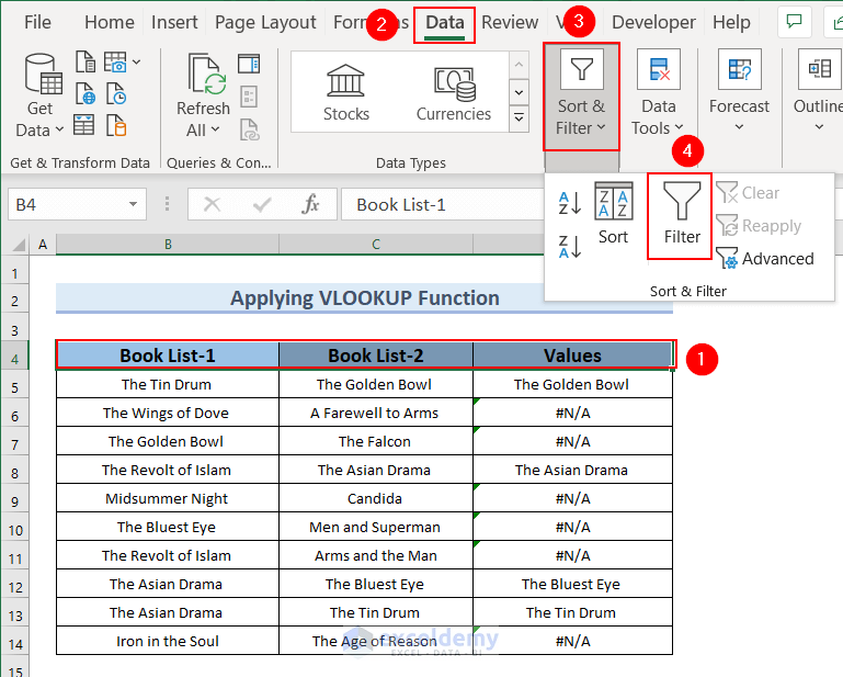
- You’ll get the Filter icon in every column of the dataset.
- Click on the drop-down icon in the Values column, and from the sorting option, check #N/A and click OK.
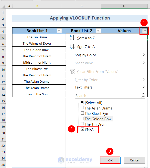
- This hides the rows that contain duplicates.
Read More: How to Remove Duplicates Using VLOOKUP in Excel
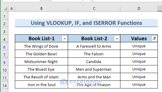
Method 5 – Integrate VLOOKUP, IF, and ISERROR Functions
Steps:
- We will use the same dataset from the previous method.
- Use the following formula in cell D5.
=IF(ISERROR(VLOOKUP(C5,$B$5:$B$14,1,FALSE)),"Unique","Duplicate")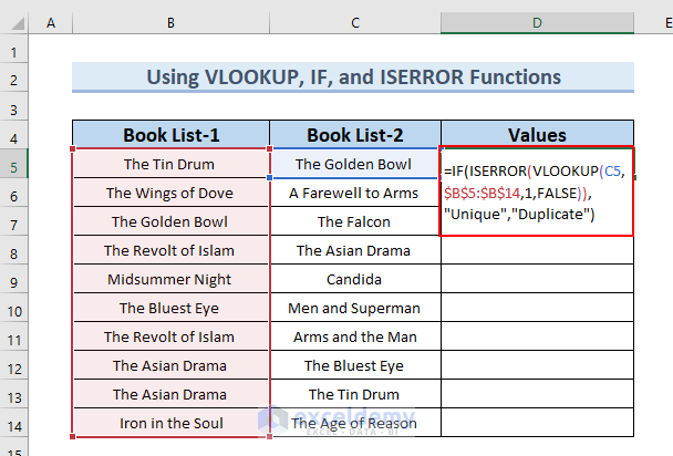
Formula Breakdown
- VLOOKUP(C5,$B$5:$B$14,1,FALSE) → this formula will find out the exact match of cell C5 value in the range of cells $B$5:$B$14. Here, Lookup_value is C5, Table_array is $B$5:$B$14. Col_index_num is 1 and [range_lookup] is (FALSE) as we want the exact match.
- IF(ISERROR(VLOOKUP(C5,$B$5:$B$14,1,FALSE)),”Unique”,”Duplicate”) → If the value is true, the formula will return “Unique”. If the value is false, the formula will return “Duplicate’’.
- Output: D5
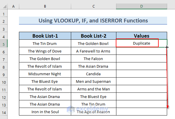
- Explanation: D5 returns Duplicate since the formula detects a duplicate value.
- Press Enter.
- Drag down the formula with the Fill Handle tool.
- Select the headings of the dataset and go to the Data tab.
- From the Sort & Filter group, select Filter.
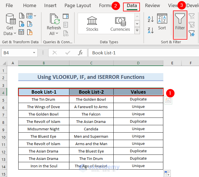
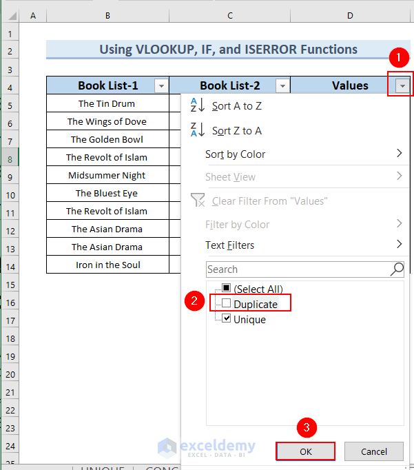
- Click on the drop-down icon of the Values columns.
- Unmark Duplicates since we want to remove them.
- Click OK.
- We only have unique values in the dataset.
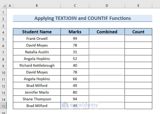
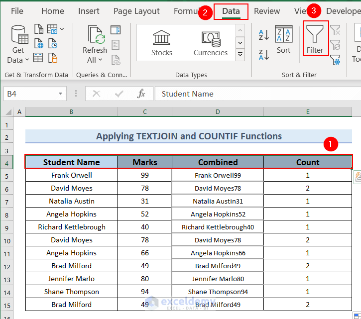
Method 6 – Use TEXTJOIN and COUNTIF Functions
We have added the Combined and Count columns in our dataset. We will use the TEXTJOIN function to find the combined values in the Combined column. After that, we will use the COUNTIF function to find the duplicate number in the Count column.
Steps:
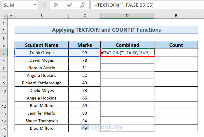
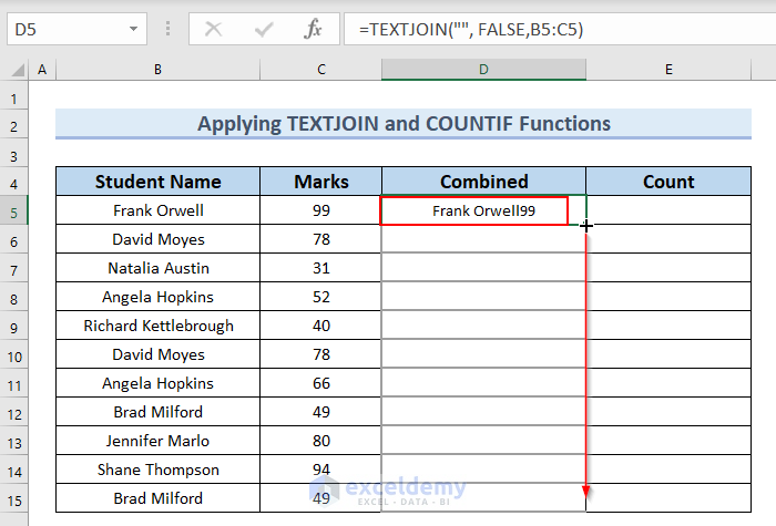
- Use the following formula in cell D5.
=TEXTJOIN("", FALSE,B5:C5)
Formula Breakdown
- TEXTJOIN(“”, FALSE,B5:C5) → the TEXTJOIN function adds text from multiple ranges.
- Output: Frank Orwell99
- Explanation: Frank Orwell99 is the combined text of cells B5 and C5.
- Hit Enter.
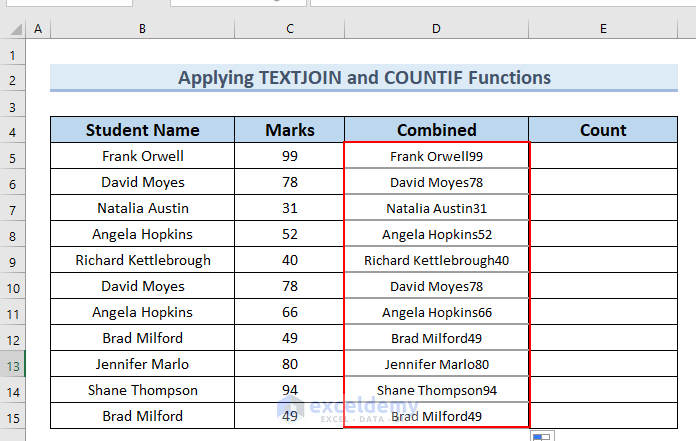
- Drag down the formula with the Fill Handle tool.
- You can see the complete Combined column.
- Use the following formula in cell E5.
=COUNTIF($D$5:$D$15,D5)The COUNTIF function counts the number of cells based on criteria.
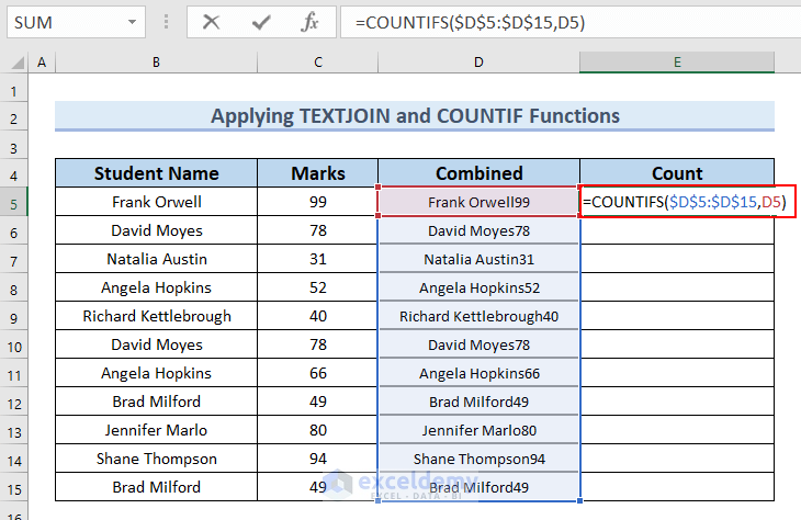
- Press Enter.
- Drag down the formula with the Fill Handle tool.
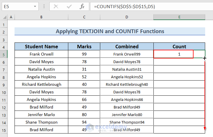
- You can see the complete Count column. In the Count column, the value is 1 for unique values and 2 for duplicate values.
- Select the headings of the dataset and go to the Data tab.
- From the Sort & Filter group, select Filter.
- Click on the drop-down icon of the Count column.
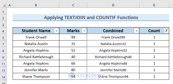
- Uncheck 2 and click OK.
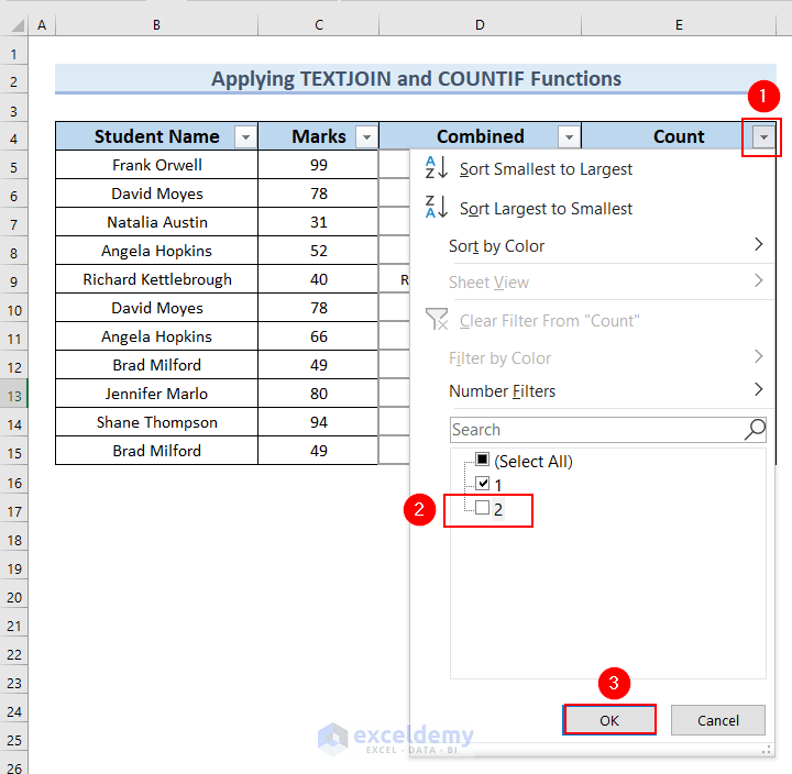
- You can see that the dataset has no duplicate values.
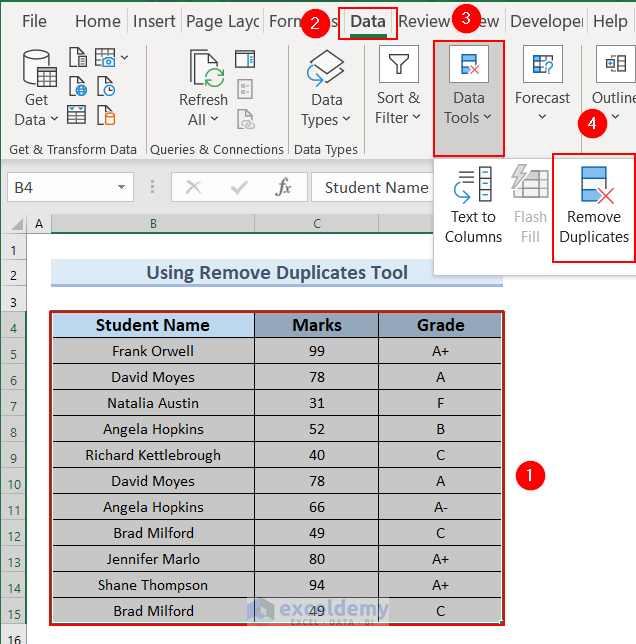
How to Remove Duplicates Using the Remove Duplicates Tool
Steps:
- Select the whole data set.
- Go to the Data tab.
- From the Data Tools group, select Remove Duplicates.
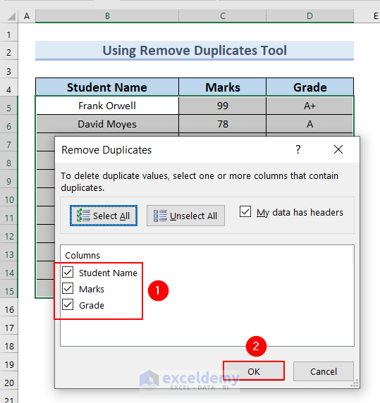
- A Remove Duplicates dialog box will appear.
- Select all the columns and click OK.
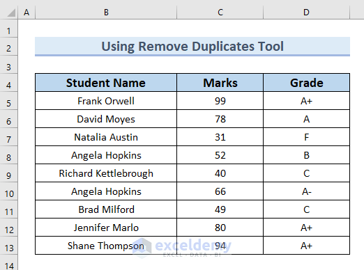
- You will get a confirmation box. Click OK.
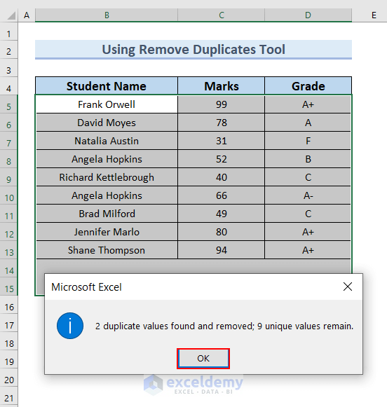
- We have removed the duplicate Student Name.
Read More: How to Find & Remove Duplicate Rows in Excel
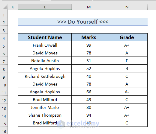
Practice Section
You can download the above Excel file and practice the explained methods.
Download the Practice Workbook
Related Articles
- How to Remove Duplicate Rows Based on One Column in Excel
- How to Remove Duplicate Rows in Excel Based on Two Columns
- How to Remove Duplicates from Columns in Excel
- Hide Duplicate Rows Based on One Column in Excel
- How to Remove Duplicate Rows in Excel Table
<< Go Back to Duplicates in Excel | Learn Excel
Get FREE Advanced Excel Exercises with Solutions!
