How to Remove Both Duplicates in Excel – 5 Easy Methods

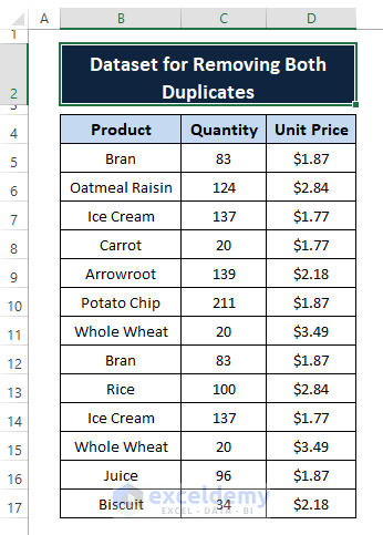
After merging data from two worksheets, the dataset contains identical entries or both duplicates:

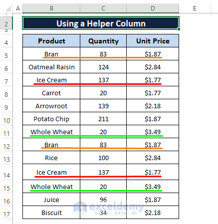
Method 1- Using a Helper Column to Remove Both Duplicates in Excel

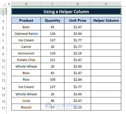
Step 1

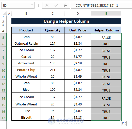
•  Insert a Helper Column (Column E).

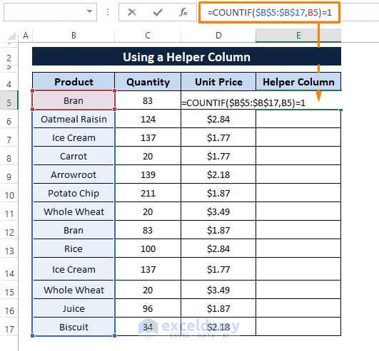
Step 2

• Enter the following formula in any cell (here, E5).

The formula counts cells in B5:B17 that match the criteria (B5) and returns TRUE (if the cell meets the criteria). Otherwise, FALSE.

 Step 3

• Press ENTER and Drag the Fill Handle to display TRUE or FALSE in the rest of the cells.

 Step 4

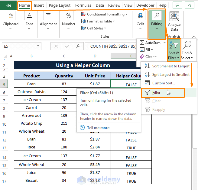
• Go to the Home Tab > Select Sort & Filter (in Editing) > Choose Filter.

Step 5

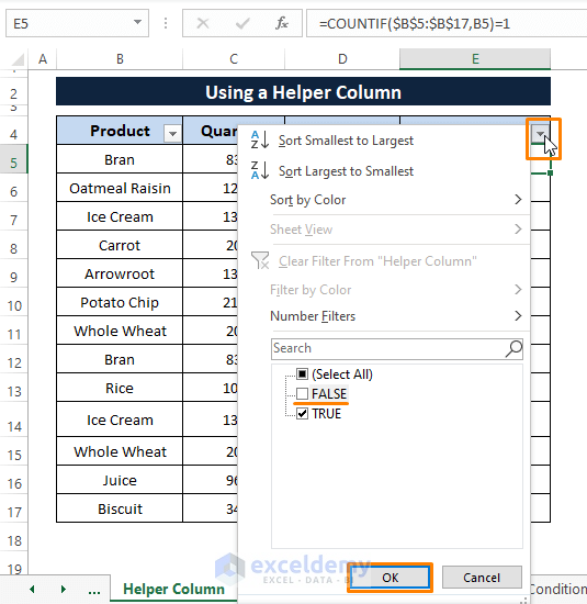
 The Filter icon is displayed in all column headers.

• Click the Filter Icon in the Helper Column header.
• Uncheck  FALSE.
• Click OK.

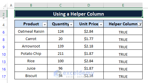
This is the output.

Method 2 – Using a Formula to Remove Both Duplicates in Excel

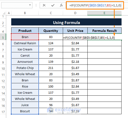
Step 1

•  Add a helper column and enter the below formula in any blank cell (here, E5).

The formula performs a logical test (i.e., COUNTIF($B$5:$B$17,B5)=1). The COUNTIF function returns TRUE or FALSE applying the criteria (iB5) in B5:B17). The IF function returns 1 if a cell meets the criteria. Otherwise, 0.

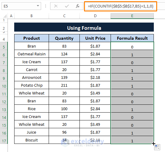
 Step 2

•  Press ENTER and drag the Fill Handle.

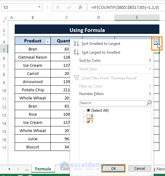
Step 3

• Apply the Filter feature: follow the steps described in Step 4 of Method 1.
• Click the Filter icon in the Formula Result column header.
• Uncheck 0.
• Click OK.

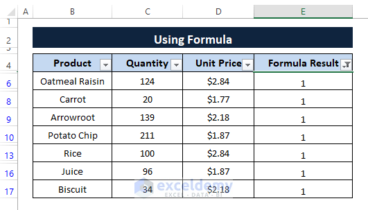
This is the output.

 In the formula ( =IF(COUNTIF($B$5:$B$17,B5)=1,1,0)) 1 are no identical entries and 0 identical entries.

Read More: How to Remove Duplicate Names in Excel

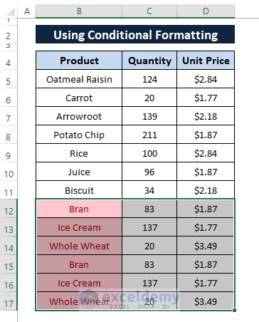
Method 3 – Using the Conditional Formatting (Highlighting Duplicates)

Step 1

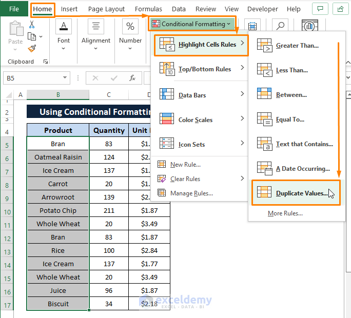
• Select the range (here, B5:B17) to apply Conditional Formatting.
• Go to the Home tab > Select Conditional Formatting > Select Highlight Cells Rules > Choose Duplicate Values.

Step 2

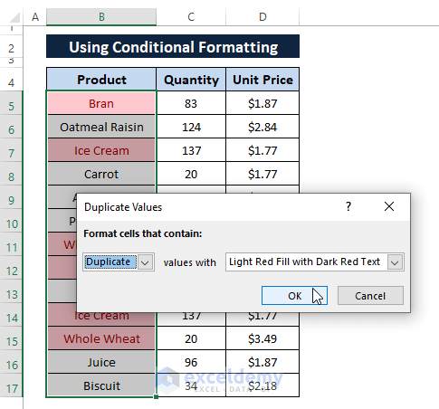
• The Duplicate Values window opens.
• Choose Duplicate (in Formats cells that contain).
• Select a Cell Color (here, Light Red Fill with Dark Red Text).
• Click OK.

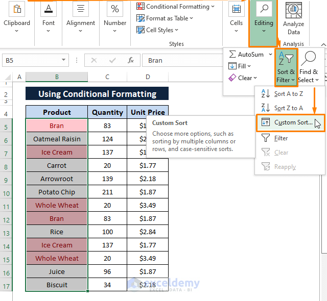
Step 3

• Go to the Home tab > Select Sort & Filter (in Editing) > Choose Custom Sort (in Sort).

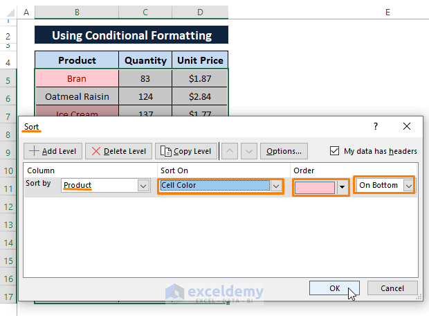
Step 4

• In the Sort window, select Product (in Column) as Sort by.
• Select a Cell Color (in Sort On).
• Select a Color in Order.
• Choose On Bottom to display the duplicates at the bottom.
• Click OK.

This is the output.

To remove the color formatted duplicates:

 a) Delete feature

• Select the color formatted cells.
• Go to the Home tab > Select Delete (in Cells) > Click Delete Sheet Rows.

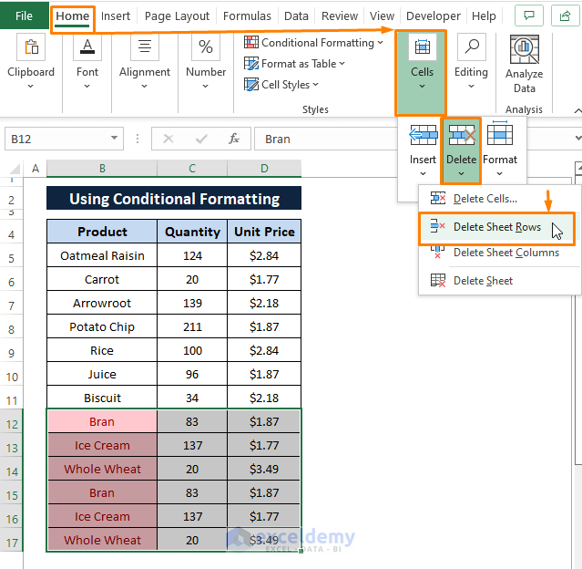
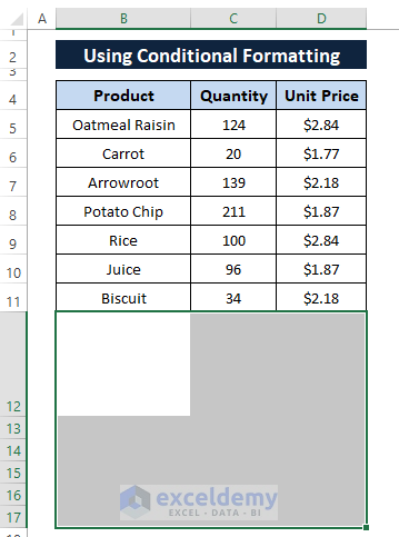
This is the output.

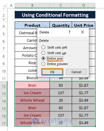
b) Keyboard Shortcuts (CTRL+-)

• Select the color formatted rows and press CTRL+- .
• In the Delete window, select Entire Row.
• Click OK.

This is the output.

c) Context Menu Delete Option

• Select the cell range and right-click it.
• In the Context Menu, select Delete.

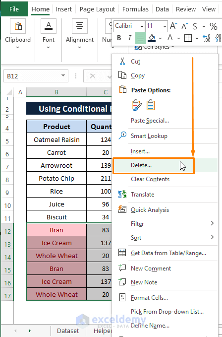
• In the Delete window, select Entire row.
• Click OK.

This is the output.

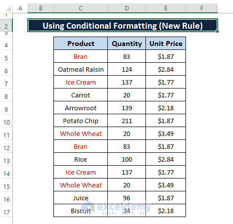
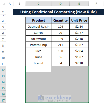
Method 4 – Using the Conditional Formatting (A New Rule to Apply Color Format)

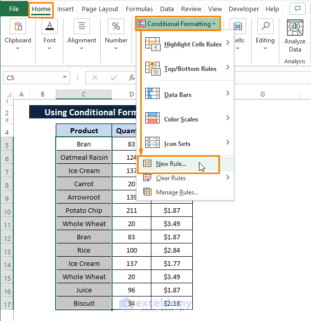
Step 1

Go to the Home tab > Select Conditional Formatting > Choose New Rule.

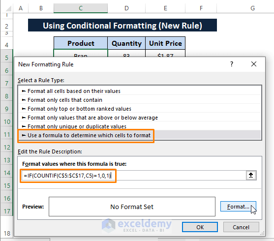
Step 2

•  In the New Formatting Rule window: select Use a formula to determine which cells to format in Select a Rule Type.
• Enter the following formula in Format values where this formula is true.

This formula declares the same arguments the one used in Step 2 of Method 1, but it returns 0 if entries meet the argument. Otherwise, 1.

• Click Format.

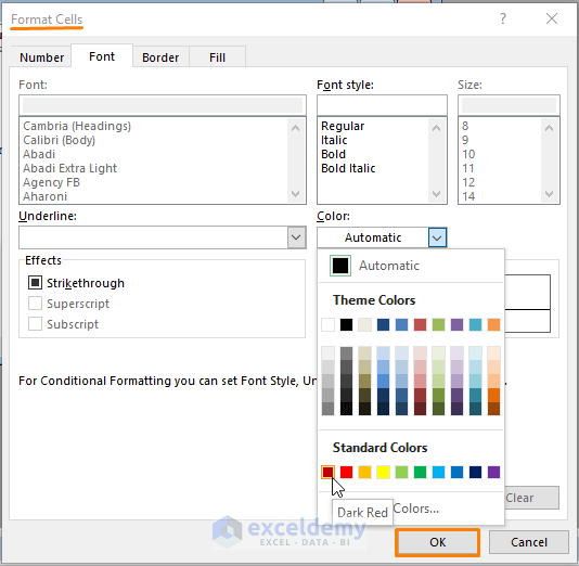
Step 3

•  In the Format Cells window, select the Font color (here, Dark Red).
• Click OK.

Step 4

•  In the New Formatting Rule window, click OK.

Step 4 applies the formula to the selection and color format to the cells.

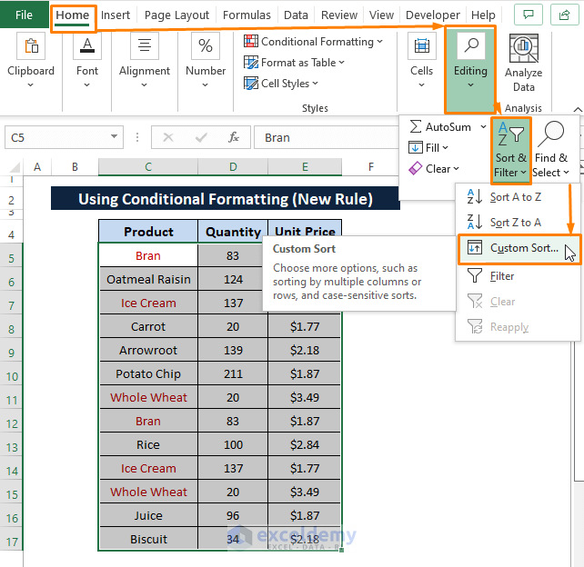
Step 5

• Select the entire dataset.
• Go to the Home tab > Select Sort & Filter (in Editing) > Choose Custom Sort. The Sort window is displayed.

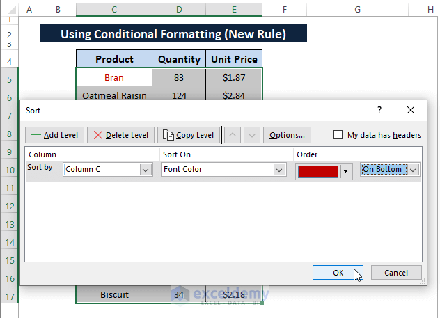
Step 6

• Enter Column C (in Column > Sort by).
• Choose a Font Color (in Sort On).
• Choose the Color in Order.
• Choose On Bottom to make the duplicates appear at the bottom.
• Click OK.

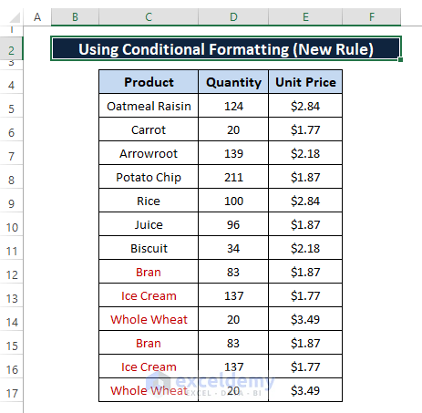
This is the output.

Step 7

Follow the steps described in Method 3 to delete cells.

This is the output.

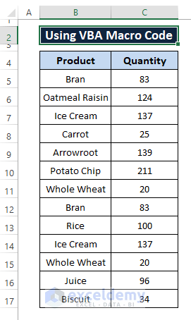
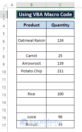
Method 5 – Using a VBA Macro Code

This is the sample dataset.

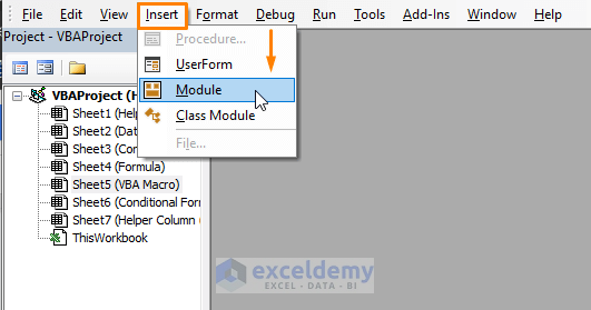
Step 1

• Press ALT+F11 to open the Microsoft Visual Basic window.
• Select Insert > Choose Module.

Step 2

• Enter the following code in the Module.

Sub Remove_Both_Duplicates()
Dim Cell As Range
With ActiveSheet.UsedRange
For Each Cell In .Cells
If Cell.Value <> "" And Application.CountIf(.Cells, Cell.Value) > 1 Then
.Replace Cell.Value, "", xlWhole, , , , False, False
End If
Next
On Error GoTo NoBlanks
End With
NoBlanks:
End Sub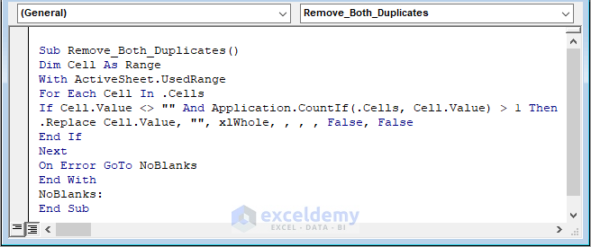

The COUNTIF function counts cells that have  more than 1 occurrences. The REPLACE function replaces the cells with blank strings.

 Step 3

• Press F5 to run the macro.
• Go back to the worksheet.

This is the output.

Download Excel Workbook

Related Articles

• How to Remove Duplicates and Keep the First Value in Excel
• Remove Duplicate Rows Except for 1st Occurrence in Excel
• How to Undo Remove Duplicates in Excel
• How to Hide Duplicates in Excel 
• How to Remove Duplicate Rows in Excel Table
• Excel Remove Duplicates Not Working 
• How to Delete Duplicates But Keep One Value in Excel 

<< Go Back to Remove Duplicates in Excel | Learn Excel