How to Remove Duplicate Names in Excel (6 Simple Methods) -

In this article, we are going to cover some easy and effective tricks on how to remove duplicate names in Excel. Sometimes, we store the same names or data in a column and later we may need to extract the unique data from that dataset.

Finding duplicate values one by one would be a time-consuming procedure, but fortunately, Excel has some lucrative features to do this job. Please follow this article to see some various ways to remove duplicate names in Excel.

You are going to have an overall idea of one procedure to remove duplicate names from rows from the following video.

Here, we removed rows that contain duplicate names. The Remove Duplicates feature was used in the video. This only returns the unique names from each row.

How to Remove Duplicate Names in Excel: 6 Easy Ways

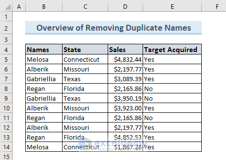
Here, we will work on the following data table. It contains the names of some salesmen, their state address and sales amount in dollars, and also their target achievement.

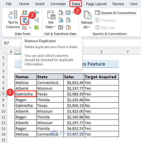
1. Using the Remove Duplicates Feature to Remove Duplicate Names from Rows in Excel

The basic way to remove duplicate names from a row is to use the Remove Duplicates feature. Please follow the procedure below to become familiar with this feature.

First, select any cell from the data table.
Next, select Data >> Remove Duplicates from the Data Tools

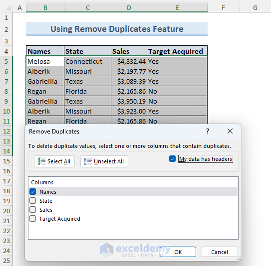
The Remove Duplicates dialog box will pop up. Check a column name on which you will operate the Remove Duplicates Make sure to select My data has headers.
After that, click OK.

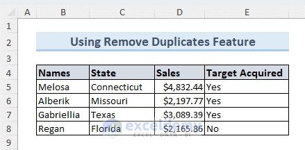
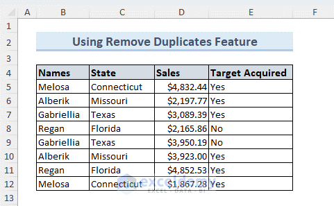
Now, all the duplicate names are removed. Only the unique names will prevail in the sheet.

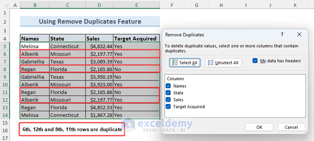
If you want to remove duplicate values based on the whole contents of the rows, you need to check all the columns. Here, the 6th and 12th rows of the sheet are exactly the same. The same can be said for the 8th and 11th rows.

The following picture shows the unique rows only.

By following the above instructions, you can remove duplicate names from rows in an Excel sheet.

Note: The command may remove some necessary data. So it is suggested that you keep a copy of your original data in your Excel workbook.

2. Remove Duplicate Names in Excel with Advanced Filter

Advanced Filter feature can also remove duplicate names from a data table. Please follow the video.

We showed the following steps in the video.

Select the Names column.
After that, go to Data >> Advanced Filter from the Sort & Filter
Check Unique records only on the Advanced Filter dialog box and click OK.

Finally, you will see all the duplicate names removed from the data table.

Here, we removed duplicate data based on Names. You can also do the same for the States column too. Hopefully, the following video will be helpful on this matter.

We removed the duplicate ‘States’ data similarly.

Note: We cannot get summarized data for each unique entry using the Advanced Filter feature.

3. Using Pivot Table to Remove Duplicate Data in Excel

PivotTable returns summarized data for each unique name. Hence, it removes duplicate data from rows.

To create a PivotTable,

First, select the whole data table.
Next, select Insert >> PivotTable.
In the PivotTable dialog box, choose the sheet where you want to keep the PivotTable. Here, we select a New Worksheet for our PivotTable.
Finally, click OK.

After that, the PivotTable will appear in a new sheet. We can make a data table without the Duplicate Names using this PivotTable. Follow the video below to understand this idea.

Here, we simply selected two columns- Names and Sales from the PivotTable Fields. The PivotTable returns the total sales done by each employee. You won’t see any duplicate names here.

Advantage: The main advantage of using PivotTable is we can get the summarized data for each entry. When we used Advanced Filter, we got the unique names that appeared first in the data table.

4. Remove Duplicate Names in Excel Using Formula

We can use formulas to remove duplicate names. I am going to show you two simple methods here.

4.1. Dynamically Remove Duplicate Names Using UNIQUE Function

In this section, we will see how to remove duplicate names using the UNIQUE function. Let’s go through the following description.

To make the procedure dynamic, convert the dataset to a table first. For this reason, select the whole data range and press Ctrl + T, make sure to check My table has headers and click OK on the dialog box (in case you forgot how to convert a dataset to an Excel table).
Select any cell where you want to keep the unique names and type the formula below.

=UNIQUE(B4:E14)

The formula will return the unique rows only.

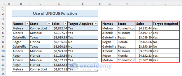
The returned range does not have any formatting. So format it according to your convenience.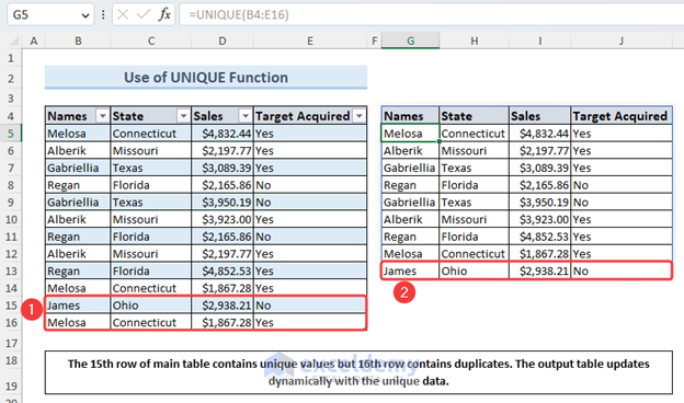

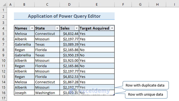
Advantage: The procedure is dynamic, once you insert a new name, it will automatically update the range that is obtained using the UNIQUE function. In the above image, we added a unique data in the 15th row and a duplicate data in the 16th row. You can see the unique data in the output range of the formula.

4.2. Remove Duplicate Names Using COUNTIF Function

You can also use the COUNTIF function to create a helper column to detect any duplicate name in a column. Let’s have a look at the description below.

In the helper column, copy the formula below and use the Fill Handle feature to AutoFill the lower cells.

=COUNTIF($B$5:B5,B5)

Now, watch the video below how we can extract the unique names applying a Filter in the data table.

The following steps were covered in the video.

Select any cell of the data table.
Press Ctrl + Shift + L to apply Filter on it.
Select the drop down icon beside the Helper column and uncheck 2 and 3.
Click OK.

You will see only the unique names after this operation.

However, Filter command doesn’t remove the duplicate names. It just hides them. To remove the duplicate names permanently, follow the video below.

In the video, the following tasks were done.

We selected the drop down icon beside the Helper column, unchecked 1 and clicked OK.
After that, the duplicate names will be filtered.
Delete these rows with duplicate names and press Ctrl + Shift + L.

Now, you will see the unique names only.

5. Use of Power Query Editor to Remove Duplicate Names

Power Query Editor is a very useful tool in Excel that provides various features to analyze the data table. We can also remove the duplicate names from a data table using the Power Query Editor.

You will find some useful instructions in the following section regarding the removal of duplicate names using the Power Query Editor. Let’s go through the description below.

First, to open the Power Query Editor, it’s good to convert your dataset to a table.
Next, select the table and go to Data >> From Table/Range.

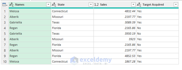
In the Power Query window, you will see the data table appear. It is accessible to various features to analyze.

The following steps were shown in the video.

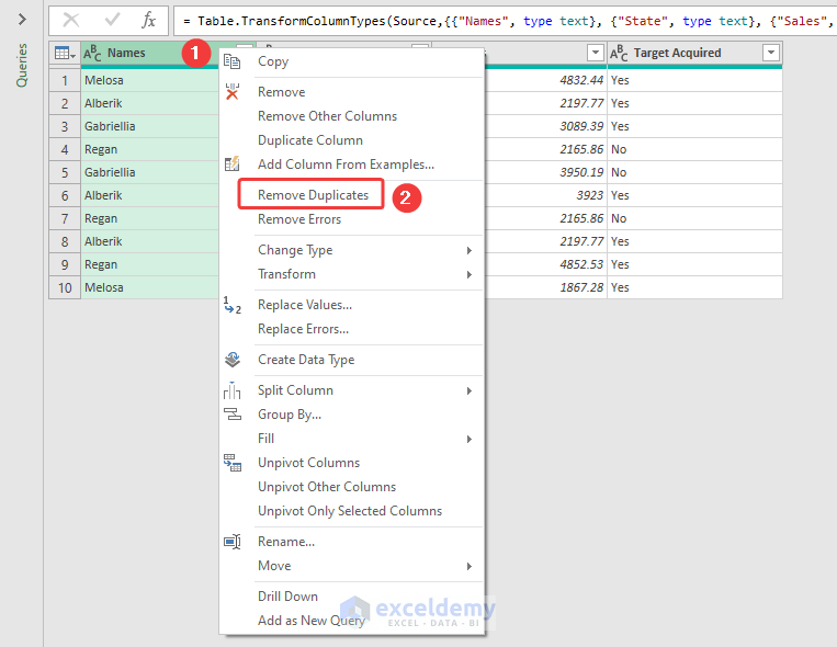
First, click on the first column name (Names).
Hold the Shift key and then click on the last column name (Target Acquired).
Next, select Remove Rows >> Remove Duplicates.
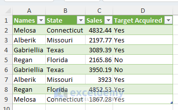
Finally, you will see only unique data in the Power Query Editor.

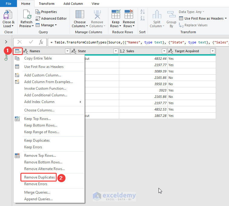
You can also remove all the Duplicate Names and data in a row from the drop down options shown in the above picture.

Now, select the Close & Load command from the Power Query ribbon. This will automatically import the data table to a new sheet.

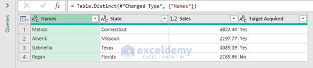
If you want to keep the unique names only and remove other duplicate names, right-click on the heading of the Names column and select Remove Duplicates.

Now, you will see the changed query with the unique names only. You can load it in a new sheet using the Close & Load command.

Advantage of Using Power Query Editor for Removing Duplicate Names

The advantage of using the Power Query Editor to remove duplicate names is that this allows us to update the table dynamically. Say, you add one duplicate and one unique data in the table. This is shown in the following image.

Now to update the data table, simply refresh it. Please follow the video below to understand this topic.

We covered the following steps in the video.

Place the cursor anywhere on the table extracted from the Power Query Editor.
Right-click and select the Refresh command from the Context Menu.

Thus your table from the Power Query Editor can be updated with the non-duplicate values.

6. Removing Duplicate Names from Single Column Using VBA

We can also use VBA to remove duplicate names. There can be several ways to remove duplicates using VBA for different situations. We’ll discuss two of the commonly used methods here.

6.1. Removing Duplicates from Fixed Cell Range

Here, we’ll show you the way of removing duplicate data from a fixed range. To open the VBA window, press Alt + F11.

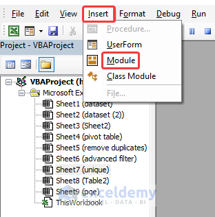
The VBA window will appear. Now, select Insert >> Module. This command will open a VBA module.

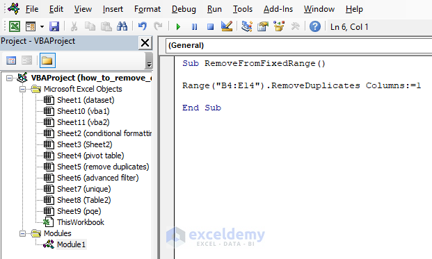
Sub RemoveFromFixedRange()
Range("B4:E14").RemoveDuplicates Columns:=1
End Sub

Now, go back to your sheet and select Developer >> Macro or press Alt + F8. Select the Macro named RemoveFromFixedRange and click OK. Follow the video below to have a better understanding on this matter.

After running the Macro, you will see the duplicate names only with their first corresponding rows.

6.2. Removing Duplicates from Selected Cell Range

You can also remove a certain amount of duplicate names and keep the other duplicate data in the data table using VBA. Let’s have a glance at the following description.

Copy the code below to a new Module.

Sub RemoveDuplicatesSelectedRange()
Dim mn_input_range As Range
Set mn_input_range = Selection
mn_input_range.RemoveDuplicates Columns:=1, Header:=xlYes
End Sub

Code Breakdown

First, a sub procedure named RemoveDuplicatesSelectedRange() is initiated.
Next, we declared a variable mn_input_range as Range.
Following that, we set the input range variable to Selection.
After that, we used the RemoveDuplicates Method to remove the duplicates from the selected range.

Finally, we run the code.

Follow the video below to see how to remove duplicates from a selected range.

Say, you want to keep the data in the first 4 rows and remove the duplicate names from the 5th row of the dataset. To do that,

First, we select the range B9:E14.
Next, we ran the Macro and removed the duplicate names from the 5th row of our dataset.

We can also introduce a Button to make our task easier. 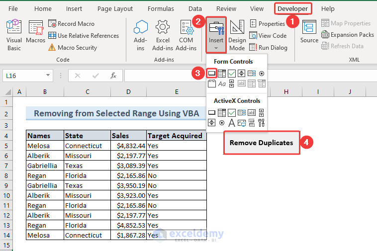Let’s have a look at the following instructions.

Select Developer >> Insert >> Button from the Form Controls
Create the button by dragging the mouse and give it a name.

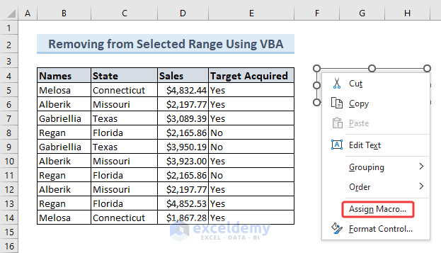
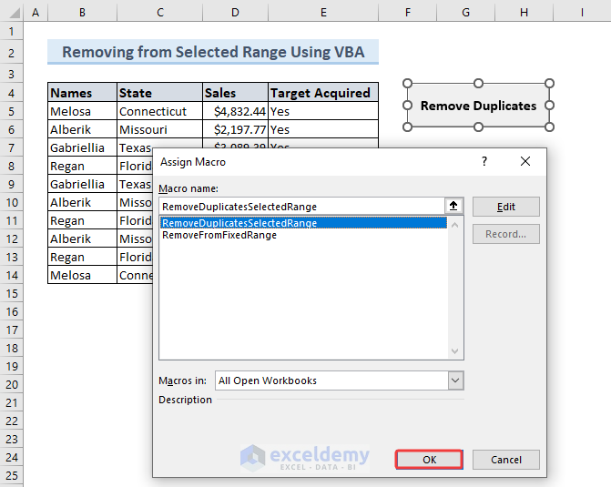
Right-click on the button and select Assign Macro from the Context Menu. You can also assign a Macro before giving the button name. But for simplicity, I’m giving you easy heads ups.

A dialog box will pop up. Assign the macro that you want to run with the button click and click OK.

Please go through the following video to see how you can run the Macro to remove duplicate names using the button click.

How to Highlight Duplicate Names in Excel

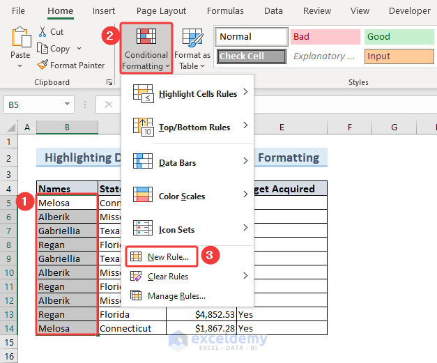
If you want to highlight duplicate names, rather than removing them, please go through the following steps.

Select the column or range where your duplicate names will be highlighted.
After that, select Conditional Formatting >> New Rule.

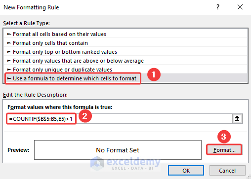
A dialog box will pop up. Select the option ‘Use a formula to determine which cells to format’ and copy the formula below to set the rule.

=COUNTIF($B$5:B5,B5)>1

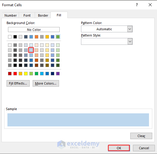
Now, select a fill color that will highlight the duplicate names and click OK.

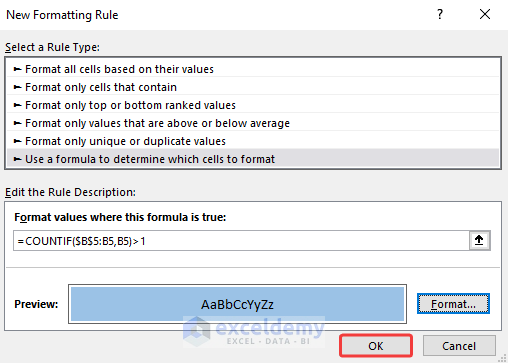
A preview will appear showing how the formatted cells will look like. Just click OK again.

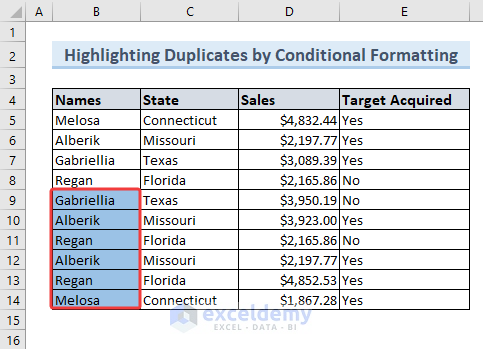
Finally, you will see the duplicate names highlighted in the data table. Thus you can apply Conditional Formatting to highlight duplicate values.

How to Keep Duplicate Rows in Excel

We have discussed various methods on how to remove duplicate names throughout this article. But sometimes, you may require to keep the duplicate data only. Here, we will show you a quick trick on how you can keep the duplicate rows.

Open the Power Query Editor with the data table. The process of opening a Power Query Editor was shown in Method 5. Follow the video below to see the steps of keeping duplicate rows in the Power Query Editor.

We showed the following steps in the video.

Select the first column heading, hold the Shift key and then select the last column heading.
After that, select Home >> Keep Rows >> Keep Duplicates.
You will see the Duplicate Rows.

Following the image above, select Close & Load command.

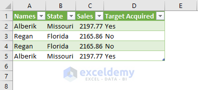
You will see a table with the duplicate names in a new sheet.

Download Practice Workbook

Remove Duplicate Names.xlsm

Conclusion

In the end, we can consider that you will learn some easy and effective tricks on how to remove duplicate names in Excel. We used different features and functions here to get this job done.

Basically, we used the Remove Duplicate feature, Advanced Filter, Power Query Editor, Formulas and VBA to remove duplicate names or contents from an Excel sheet. The Power Query Editor and Formulas can be dynamic which makes them better choice to apply.

If you have any ideas or questions or ideas regarding this article, please leave them in the comment section. This will help me enrich my upcoming articles.

<< Go Back to Remove Duplicates in Excel | Duplicates in Excel | Learn Excel

Get FREE Advanced Excel Exercises with Solutions!

How to Remove Duplicate Names in Excel (6 Simple Methods)