Method 1 – Hide Duplicate Rows Based on One Column in Excel Using the Advanced Filter
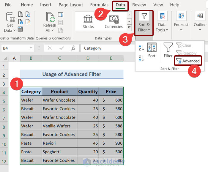
- Select the dataset.
- Go to Data, then to Sort & Filter, and choose Advanced.
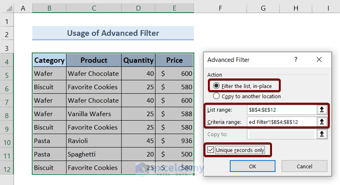
The Advanced Filter dialog box will appear.
- Select Filter the list in place.
- Insert the entire table range in the List range box.
- Insert the cell range of the first column which is B4:B12 in the Criteria range box.
- Select Unique records only and hit OK.
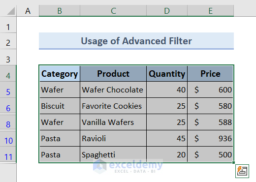
This will automatically hide the duplicate rows based on the selected column.
Read More: How to Remove Duplicates Based on Criteria in Excel
Method 2 – Use Conditional Formatting New Rule to Hide Duplicate Rows Based on One Column in Excel
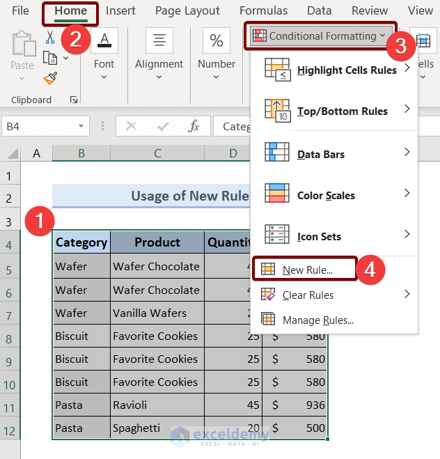
- Select the dataset.
- Go to Home, then to Conditional Formatting, and choose New Rule.
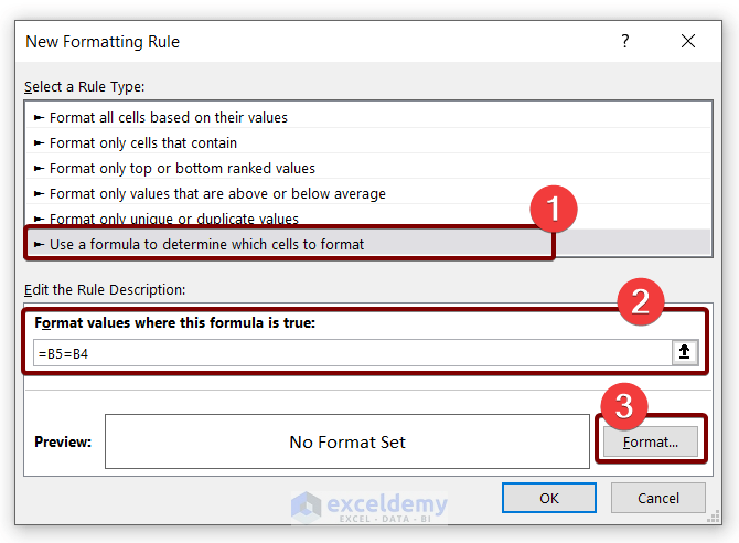
A New Formatting Rule dialog box will appear.
- Select Use a formula to determine which cells to format.
- Insert the following formula in the Format values where this formula is true box.
=B5=B4- Click on the Format button.
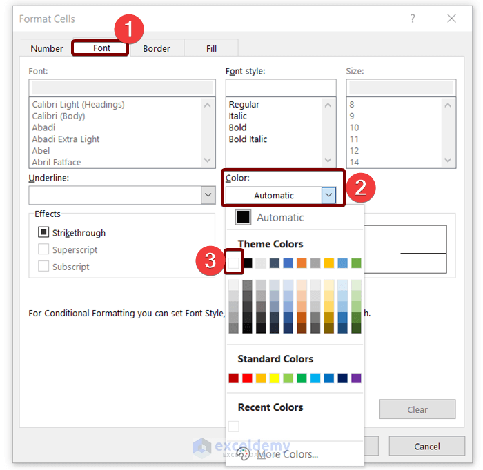
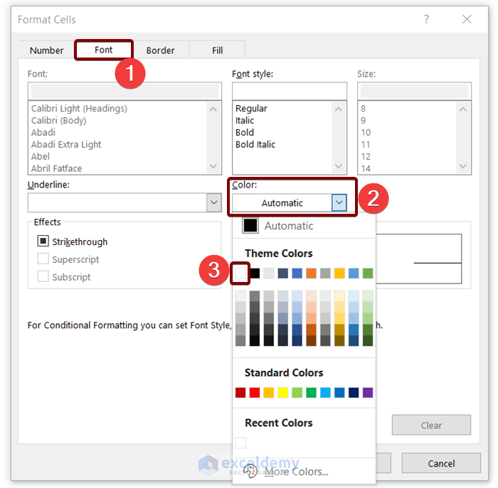
Format Cells dialog box will appear.
- Go to the Font tab.
- Select White in the Color section and hit OK.
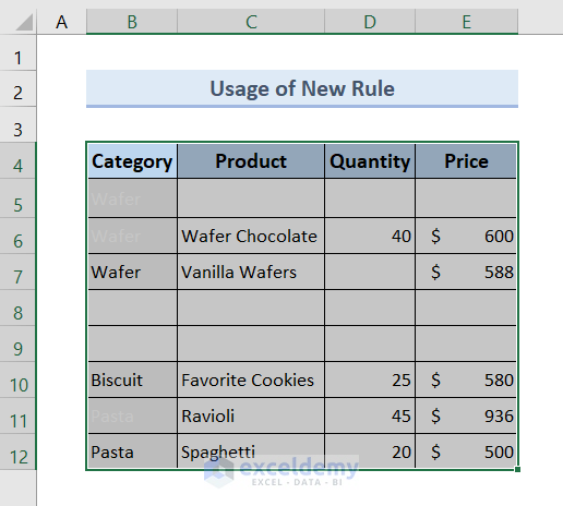
All the duplicate rows will be hidden based on the previous column.
Read More: How to Hide Duplicates in Excel
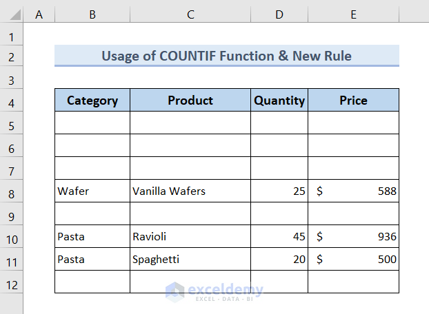
Method 3 – Hide Duplicate Rows Based on One Column Using the COUNTIF Function and New Rule in Excel
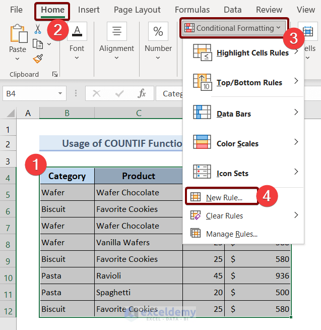
- Select your data table.
- Go to Home, then to Conditional Formatting, and choose New Rule.
A New Formatting Rule dialog box will appear.
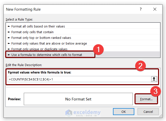
- Select Use a formula to determine which cells to format.
- Insert the following formula in the Format values where this formula is true box.
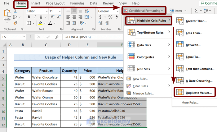
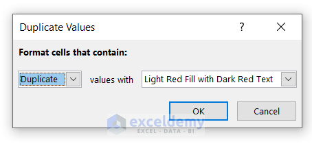
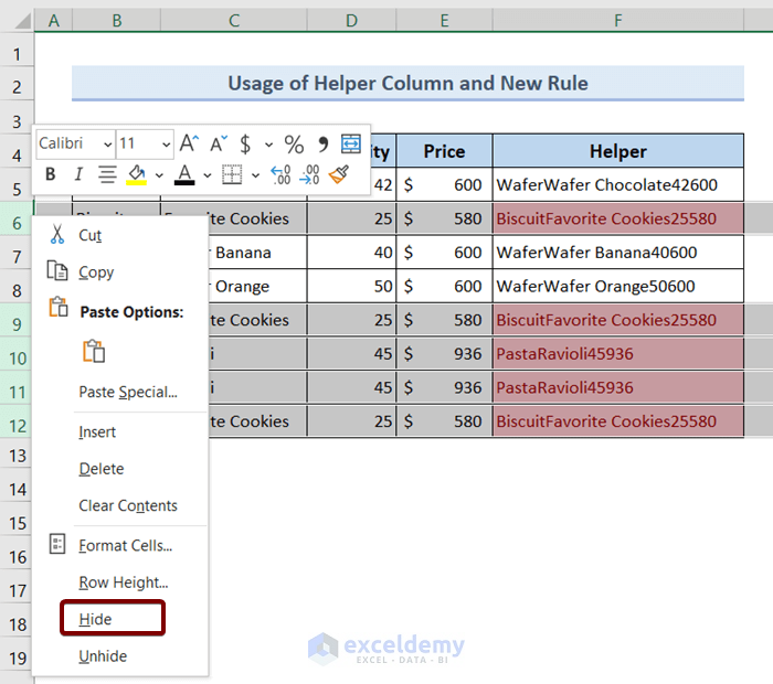
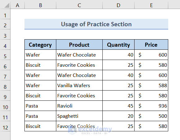
=COUNTIF($C$4:$C$12,$C4)>1Formula Explanation The COUNTIF function compares $C4 with the range $C$4:$C$12. If the result is larger than 1, that’s a duplicate entity. The Format Cells dialog box will appear. All the duplicate rows will be hidden based on the first column. Read More: How to Use Formula to Automatically Remove Duplicates in Excel The Duplicate Values dialog box will appear. All the duplicate values will be marked in red color. All the duplicate rows will be hidden. Read More: How to Find & Remove Duplicate Rows in Excel You will get an Excel sheet like the following screenshot at the end of the provided Excel file, where you can practice all the methods discussed in this article. Download the Practice Workbook << Go Back to Duplicates in Excel | Learn Excel
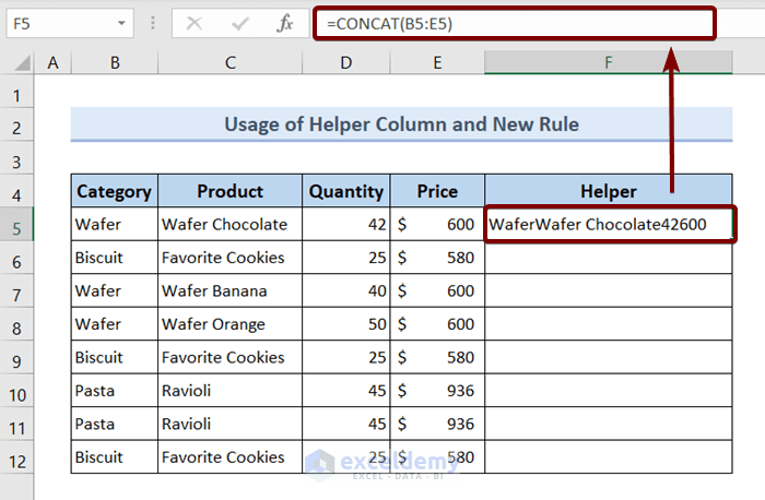
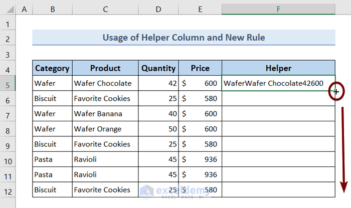
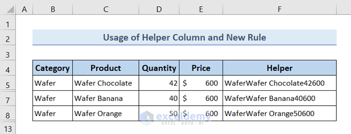
Method 4 – Use the CONCAT Function and the Context Menu to Hide Duplicate Rows Based on One Column
=CONCAT(B5:E5)
Practice Section
Related Articles

