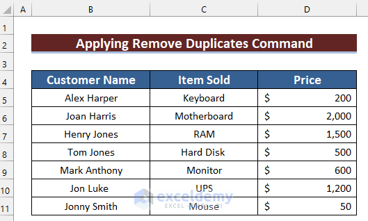
The following dataset contains “Customer Name” and “Item Sold” columns. There are duplicate values.
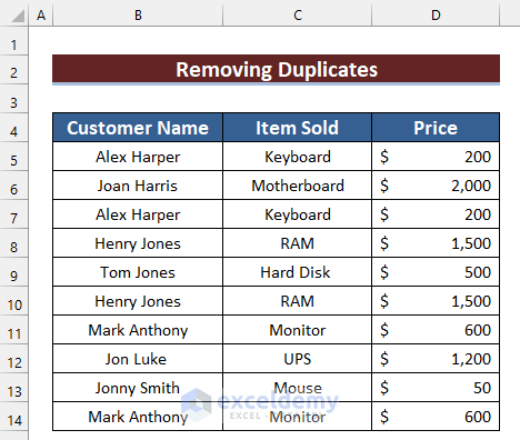
Method 1 – Using an Advanced Filter to Remove Duplicates Based on Criteria in Excel
Steps:
- Slect the cell range in which you want to remove duplicates. Here, B4:D14.
- Go to the Data tab.
- Select Advanced.
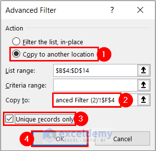
- In the Advanced Filter dialog box, select Copy to another location.
- Select the location for the copied data.
- Check Unique records only.
- Click OK.
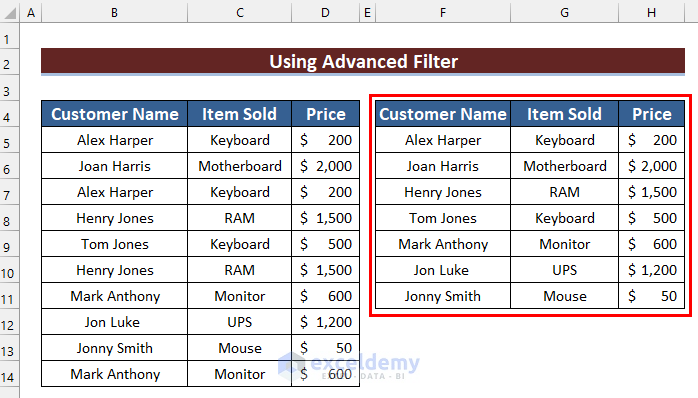
- The duplicates are removed from the dataset.
Method 2 – Using the COUNTIF Function to Remove Duplicates Based on Criteria in Excel
Steps:
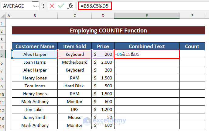
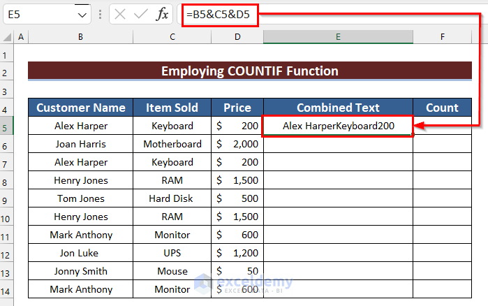
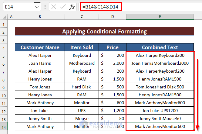
- Select the cell in which you want the Combined Text from the three columns.
- Enter the following formula.
=B5&C5&D5- Press Enter.
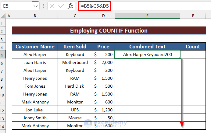
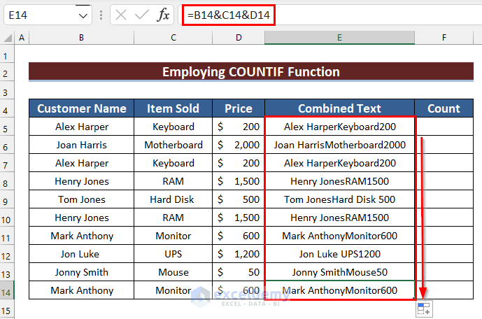
- Drag down the Fill Handle.
- The formula was copied to the other cells.
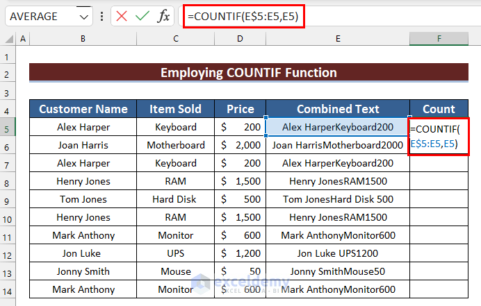
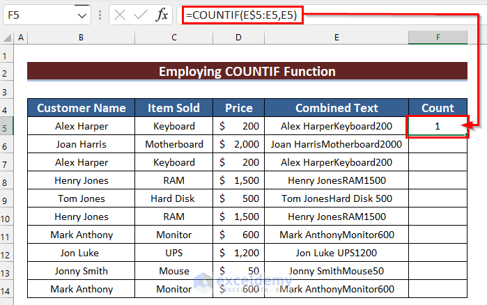
- Select the cell in which you want to Count the repeated values. Here, F5.
- In F5 enter the following formula.
=COUNTIF(E$5:E5,E5)- Press Enter to see the result.
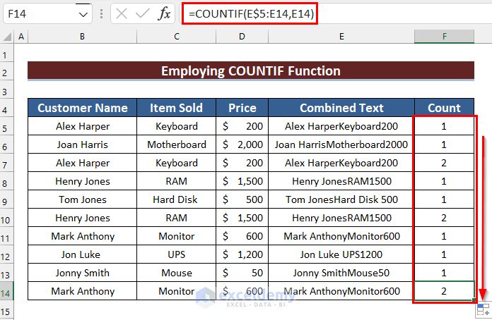
- Drag down the Fill Handle to copy the formula to the other cells.
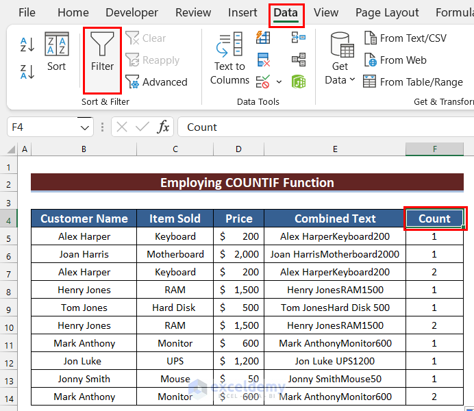
- Select the column header of the Count column.
- Go to the Data tab.
- Select Filter.
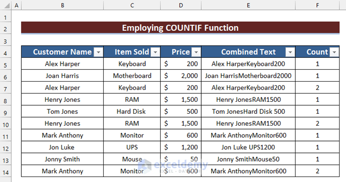
- Filter is added.
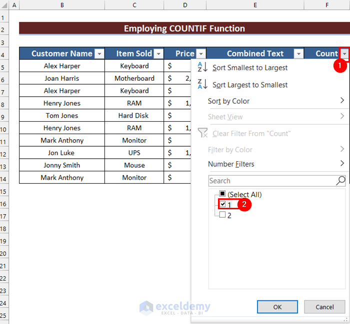
- Click the filter button.
- Check 1.
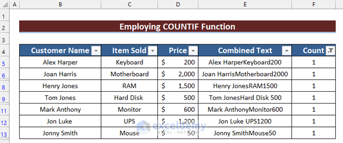
- Duplicate rows are removed from the dataset.
Read More: How to Use Formula to Automatically Remove Duplicates in Excel
Method 3 – Applying the Remove Duplicate Command Based on Criteria in Excel
STEPS:
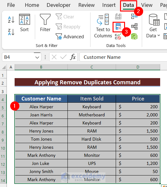
- Select the cell range for your dataset. Here, B4:D14.
- Go to the Data tab.
- Select Remove Duplicates.
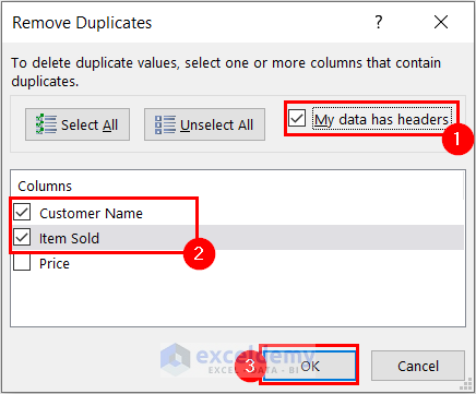
- The Remove Duplicates dialog box will open.
- Check My data has headers.
- Select the Columns in which you want to remove data.
- Click OK.
- A message will be displayed.
- Click OK.
- The duplicates are removed from the list.
Read More: How to Remove Duplicate Rows Based on One Column in Excel
Method 4 – Utilizing the IF and COUNTIFS Functions to Remove Duplicates Based on Criteria
Example1: Keep First Data and Remove Other Duplicates
Steps:
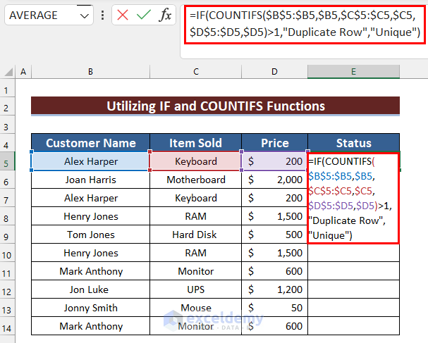
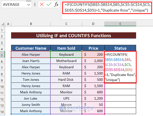
- Select the cell in which you want to remove duplicates.
- Enter the following formula.
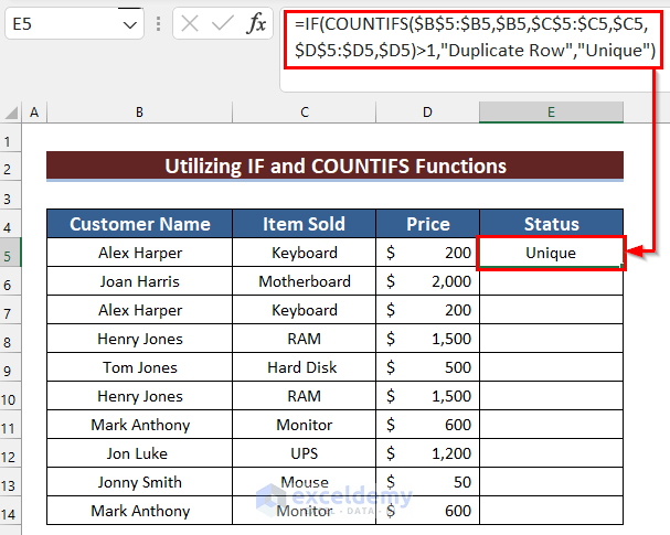
=IF(COUNTIFS($B$5:$B5,$B5,$C$5:$C5,$C5,$D$5:$D5,$D5)>1,"Duplicate Row","Unique")- Press Enter to see the result.
Formula Breakdown
- COUNTIFS($B$5:$B5,$B5,$C$5:$C5,$C5,$D$5:$D5,$D5): $B$5:$B5 is the criteria_range1, $B5 is the criteria1, $C$5:$C5 is the criteria_range2, $C5 is the criteria2, $D$5:$D5 is the criteria_range3, and $D5 is the criteria3. The formula returns the number of cells in which all criteria are met.
- IF(COUNTIFS($B$5:$B5,$B5,$C$5:$C5,$C5,$D$5:$D5,$D5)>1,”Duplicate Row”,”Unique”): checks the logical_test. If the test is True, it returns “Duplicate Row”. Otherwise, it returns “Unique”.
- Drag down the Fill Handle to copy the formula.
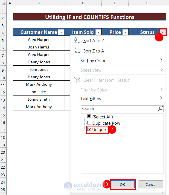
- Add Filter by following the steps in Method 2.
- Click Filter.
- Select Unique.
- Click OK.
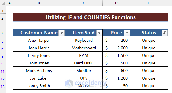
- Duplicates were removed and the first data was kept.
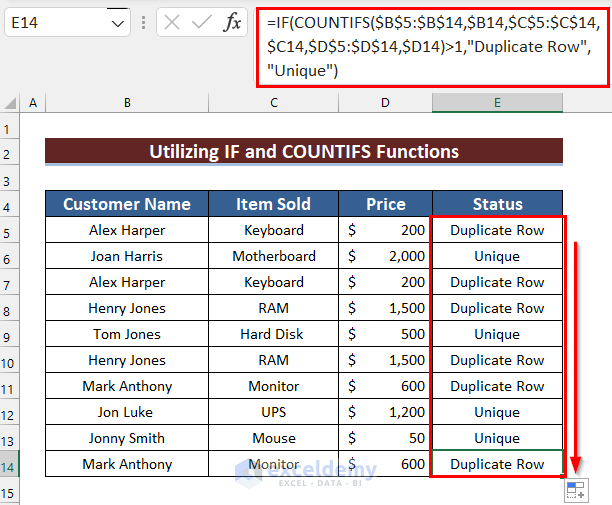
Example 2: Remove All Duplicates
Steps:
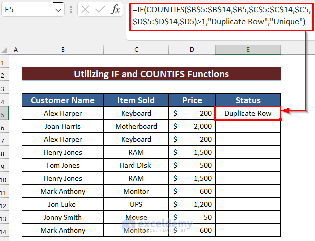
- Select the cell in which you want to remove duplicates. Here, E5.
- Enter the following formula.
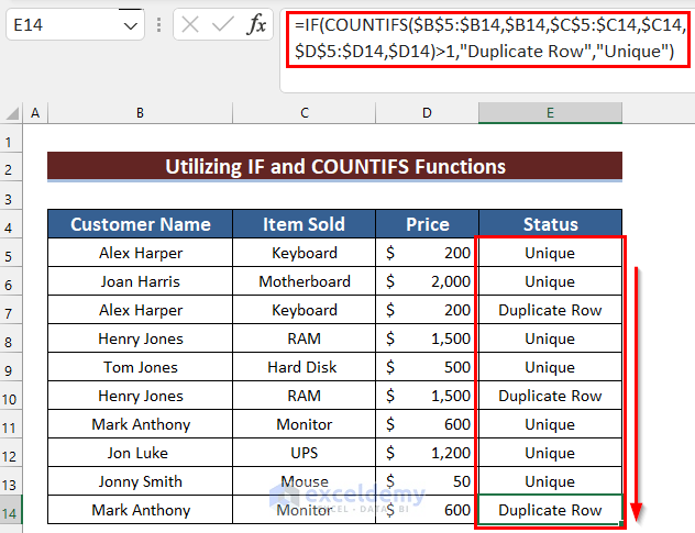
=IF(COUNTIFS($B$5:$B$14,$B5,$C$5:$C$14,$C5,$D$5:$D$14,$D5)>1,"Duplicate Row","Unique")- Press Enter to see the result.
Formula Breakdown
- COUNTIFS($B$5:$B$14,$B5,$C$5:$C$14,$C5,$D$5:$D$14,$D5): $B$5:$B$14 is the criteria_range1, $B5 is the criteria1, $C$5:$C$14 is the criteria_range2, $C5 is the criteria2, $D$5:$D$14 is the criteria_range3, and $D5 is the criteria3. The formula returns the number of cells in which all criteria are met.
- IF(COUNTIFS($B$5:$B$14,$B5,$C$5:$C$14,$C5,$D$5:$D$14,$D5)>1,”Duplicate Row”,”Unique”): checks the logical_test. If the test is True then it returns “Duplicate Row”. Otherwise, it returns “Unique”.
- Drag down the Fill Handle to copy the formula to the other cells.
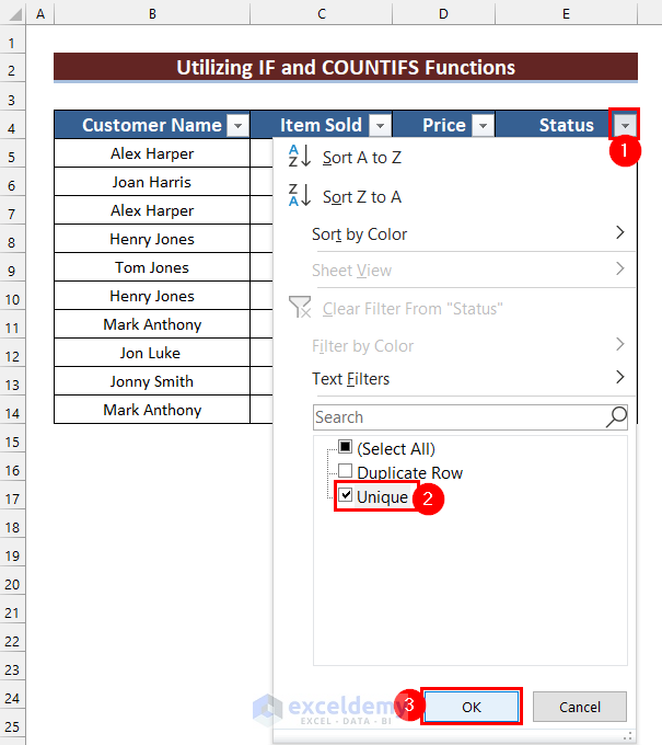
- Add Filter by following the steps in Method 2.
- Click Filter.
- Select Unique.
- Click OK.
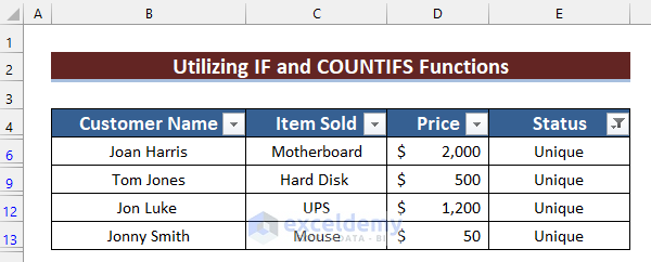
- Duplicates are removed from the list.
Read More: How to Remove Duplicates from Columns in Excel
Method 5 – Applying Conditional Formatting to Remove Duplicates Based on Criteria in Excel
Steps:
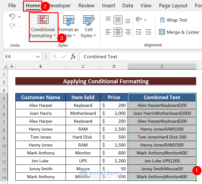
- Get the Combined Text by following the steps in Method 2.
- Select the Combined Text.
- Go to the Home tab.
- Select Conditional Formatting.
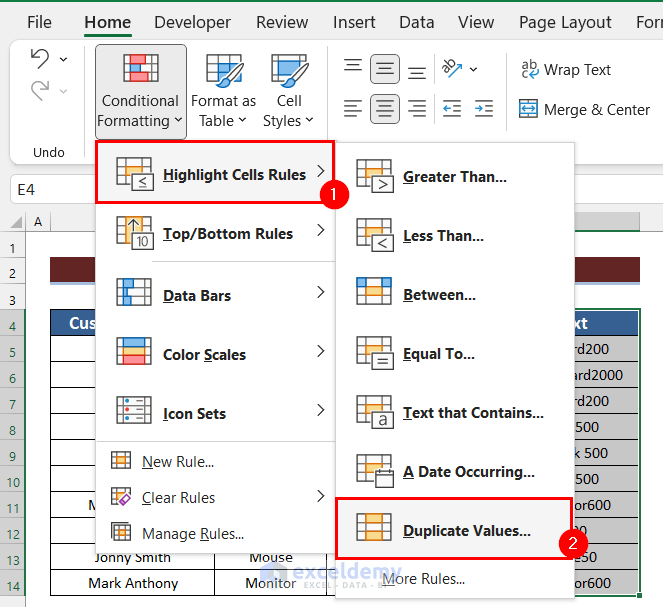
- From the drop-down menu, select Highlight Cells Rules.
- Choose Duplicate Values.
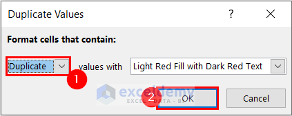
- In the Duplicate Values dialog box, select Duplicate.
- Click OK.
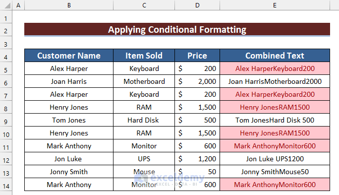
- Duplicate values are highlighted.
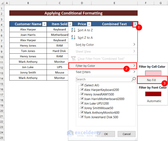
- Add Filter by following the steps in Method 2.
- Click Filter.
- Select Filter by Color.
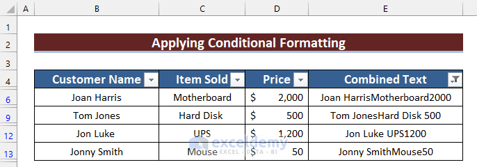
- Choose No Fill.
- Duplicates are removed from the list.
Read More: How to Remove Duplicate Rows in Excel Based on Two Columns
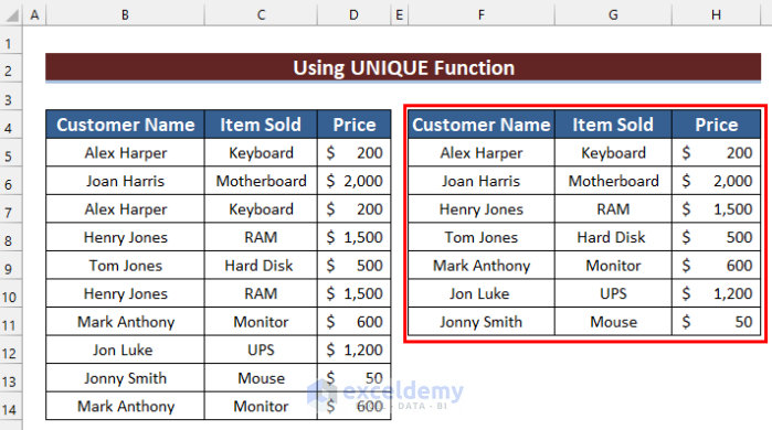
Method 6 – Using the Excel UNIQUE Function to Remove Duplicates Based on Criteria
STEPS:
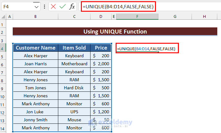
- Select the cell in which you want the unique list. Here, F4.
- Enter the following formula.
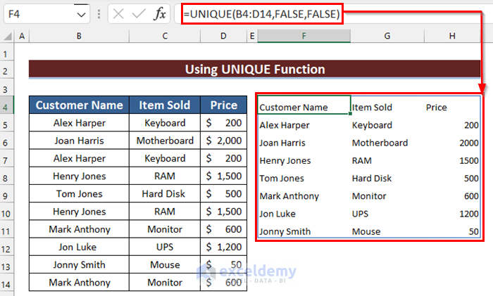
=UNIQUE(B4:D14,FALSE,FALSE)- Press Enter to see the unique list.
- Format the unique list:
Method 7 – Utilizing VBA Codes to Remove Duplicates Based on Criteria
Steps:
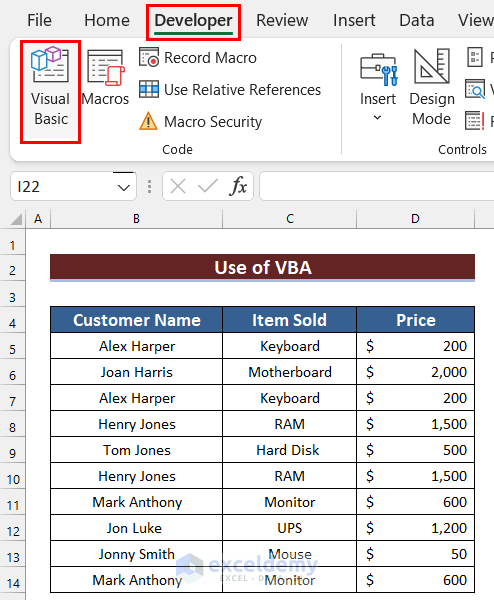
- Go to the Developer tab.
- Select Visual Basic.
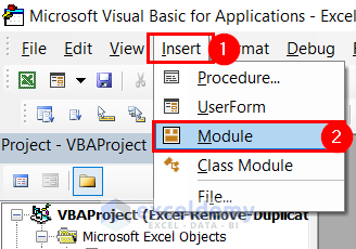
- In the Visual Basic Editor window, select Insert.
- Choose Module.
- In Module, enter the following code.
Sub Removing_duplicate_rows()
Dim selected_rng As Range
Set selected_rng = Selection
selected_rng.RemoveDuplicates Columns:=Array(1), Header:=xlYes
End Sub
Code Breakdown
- A Sub Procedure (Removing_duplicate_rows) is created.
- selected_rng as Range is declared as the variable.
- Set Statement sets the selected_rng as Selection.
- RemoveDuplicates Method removes duplicate rows in the selected range.
- End Sub Procedure.
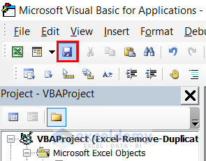
- Save the code and go back to your worksheet.
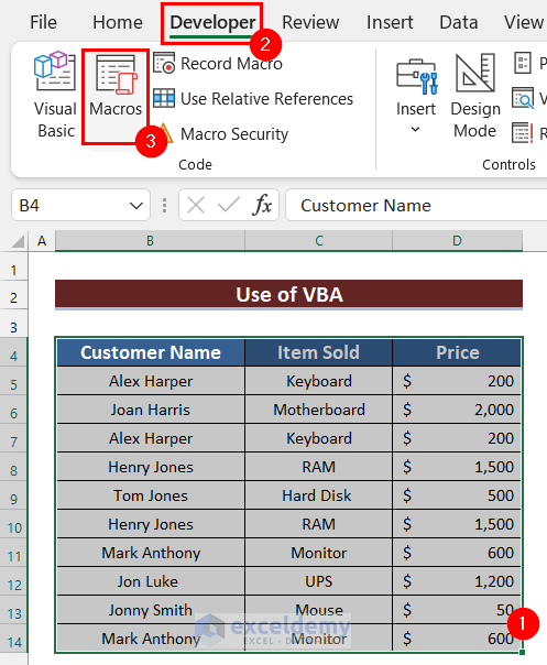
- Select the data range from which you want to remove duplicates.
- Go to the Developer tab.
- Select Macros.
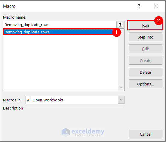
- Select Removing_duplicate_rows as Macro name.
- Click Run.
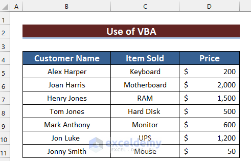
- Duplicate rows are removed from the data range.
Practice Section
Practice here.
Download Practice Workbook
Download this practice workbook to exercise.
Related Articles
- How to Find & Remove Duplicate Rows in Excel
- Hide Duplicate Rows Based on One Column in Excel
- How to Remove Duplicates Using VLOOKUP in Excel
- How to Remove Duplicate Rows in Excel Table
<< Go Back to Remove Duplicates in Excel | Learn Excel
Get FREE Advanced Excel Exercises with Solutions!




Great vba code to remove duplicates
Thanks, SANDEEP! Best regards!