Dataset Overview
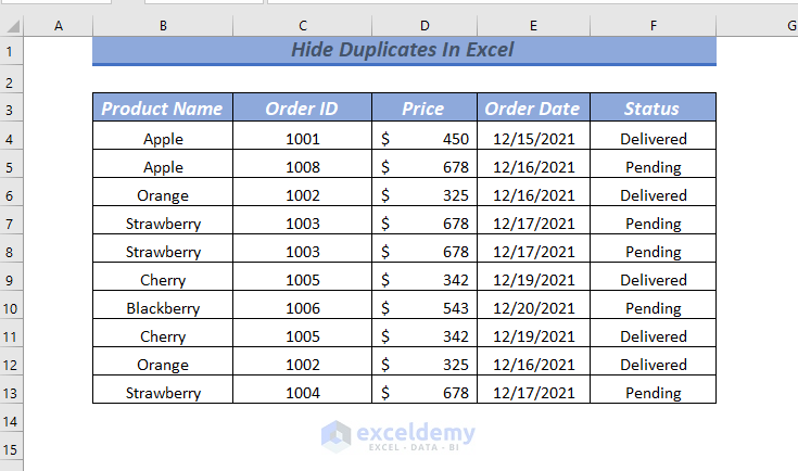
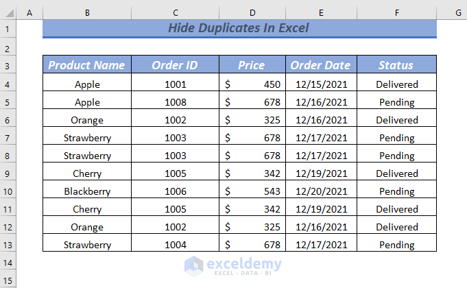
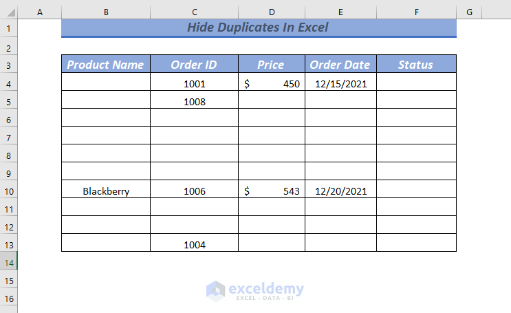
To explain this process clearly, let’s use a sample dataset from an online fruit store. The dataset contains 5 columns representing fruit order and delivery details: Product Name, Order ID, Price, Order Date, and Status.
Method 1 – Using Advanced Filter to Hide Duplicate Rows
If you have duplicate rows in your sheet, follow these steps:
- Select the range B4:F13.
- Go to the Data tab and choose Advanced.
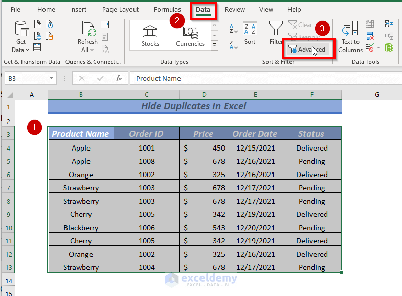
- A dialog box will appear.
- Under Action, select Filter the list, in-place.
- In the List range, ensure that B3:F13 is selected.
- Check the box for Unique records only.
- Click OK.

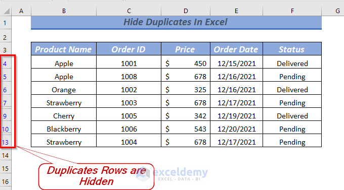
As a result, all duplicate rows will be hidden in the dataset.
If you need to unhide the duplicate rows later:
- Go to the Data tab.
- Select Clear.
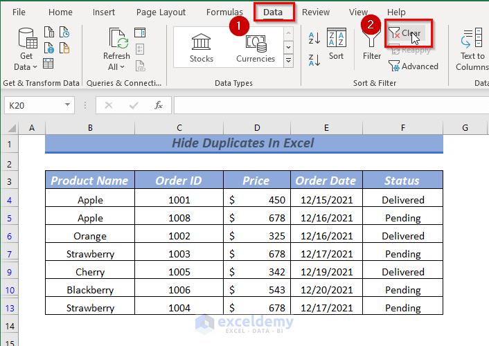
This will clear the applied Advanced Filter, and your duplicate rows will reappear.
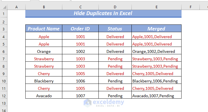
Method 2 – Using COUNTIF & Context Menu to Hide Duplicates in Excel
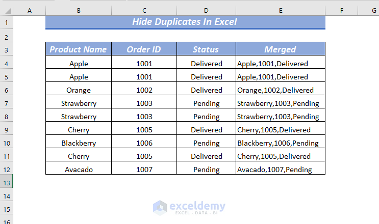
- Begin by making adjustments to your dataset. Keep the Product Name, Order ID, and Status columns, and merge them if necessary to provide a clear view of duplicate rows.
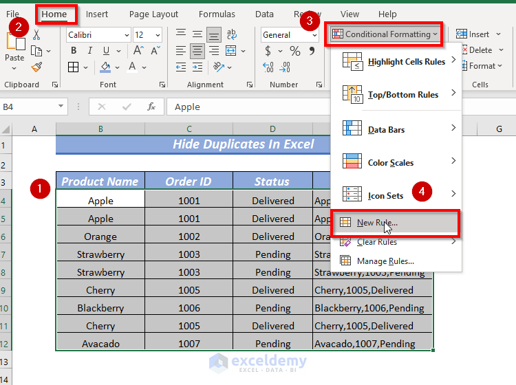
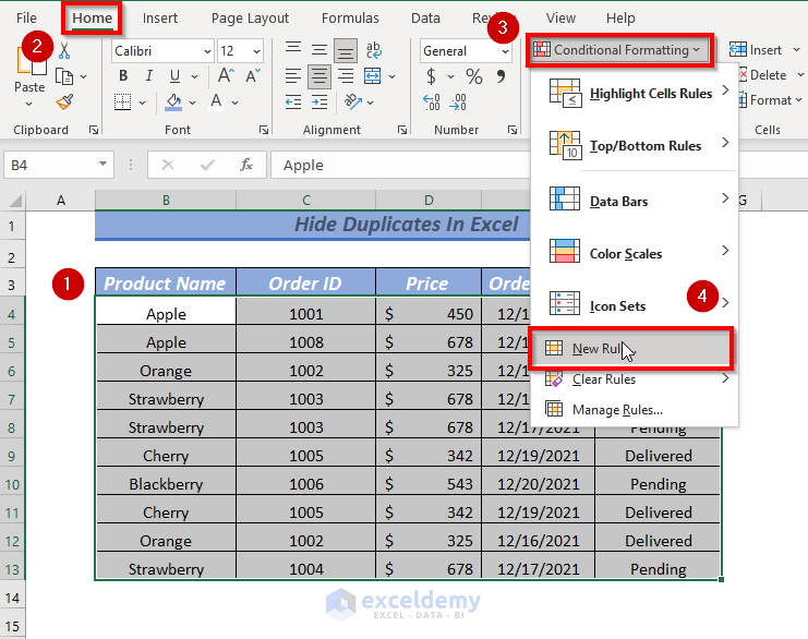
- Select the cell range where you want to apply the formatting formula. For example, choose the cell range B4:E12.
- Go to the Home tab and click on Conditional Formatting, then select New Rule.
- In the dialog box that appears:
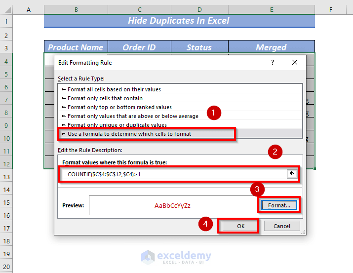
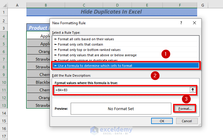
- Choose Use a formula to determine which cells to format under Select a Rule Type.
- In the Edit the Rule Description field, enter the following formula:
=COUNTIF($C$4:$C$12,$C4)>1-
-
- Here, the COUNTIF function checks if the value in cell $C4 occurs more than once within the range $C$4:$C$12.
-
- Click on Format to choose the formatting style. For example, select the color Red to format the cell values.
- Click OK.
- As a result, all duplicate values will be formatted according to your chosen style.
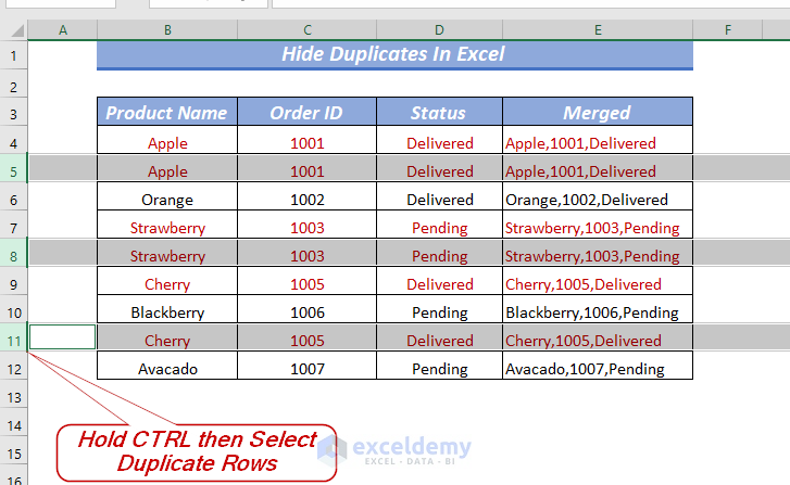
- To hide the duplicate rows using the context menu:
- Select any duplicate cell.
- While holding the CTRL key, select other duplicate rows that you want to hide.
-
- Right-click the mouse and choose Hide.
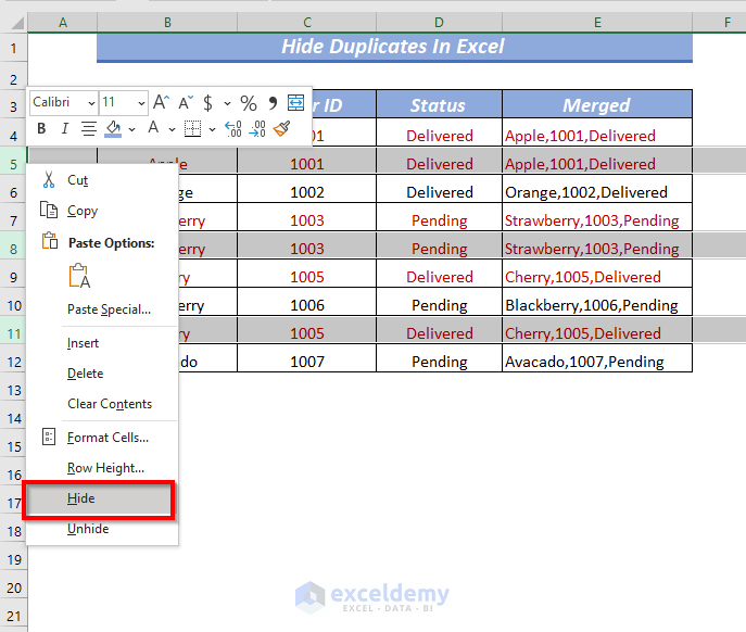
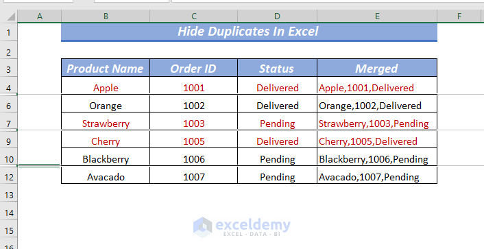
This will hide all the selected duplicate rows in your dataset.
Method 3 – Using Conditional Formatting to Hide Duplicates
The Conditional Formatting feature in Excel offers various options, and working with duplicate values is one of them.
Let’s see how you can hide duplicates using the Highlight Cells Rules:
- Select the cell range where you want to apply Conditional Formatting. For example, choose the cell range B4:F13.
- Follow these steps:
- Open the Home tab.
- Under Conditional Formatting, go to Highlight Cells Rules and select Duplicate Values.
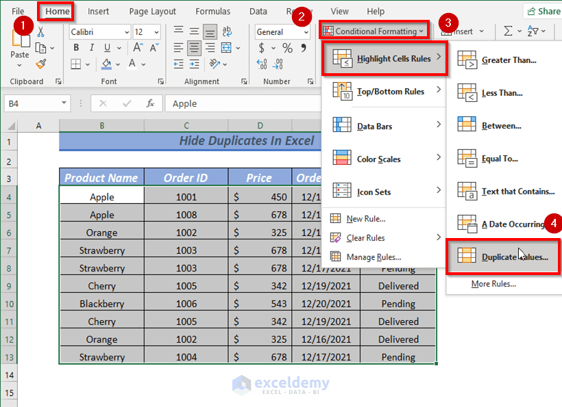
- A dialog box will appear.
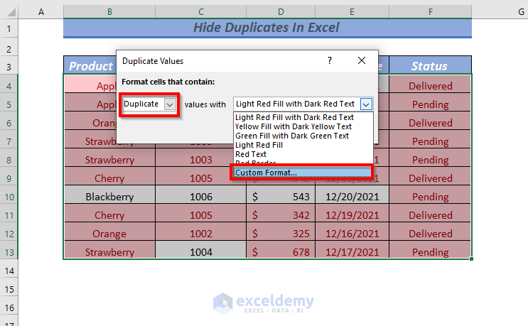
- In the dialog box:
- Choose Format cells that contain and values with.
- For Format cells that contain, select Duplicates.
- For Custom Format, another dialog box will pop up to choose the format.
- In the second dialog box, you can select any color. However, to hide duplicates, choose the same background color as your cell.
- For example, if your cell color is White, select White as the format color.
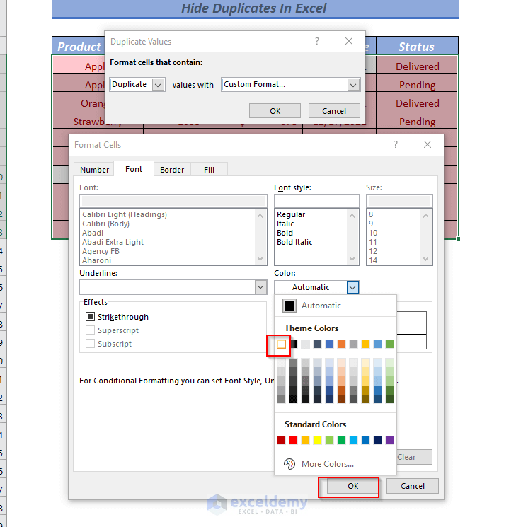
- Click OK on both dialog boxes.
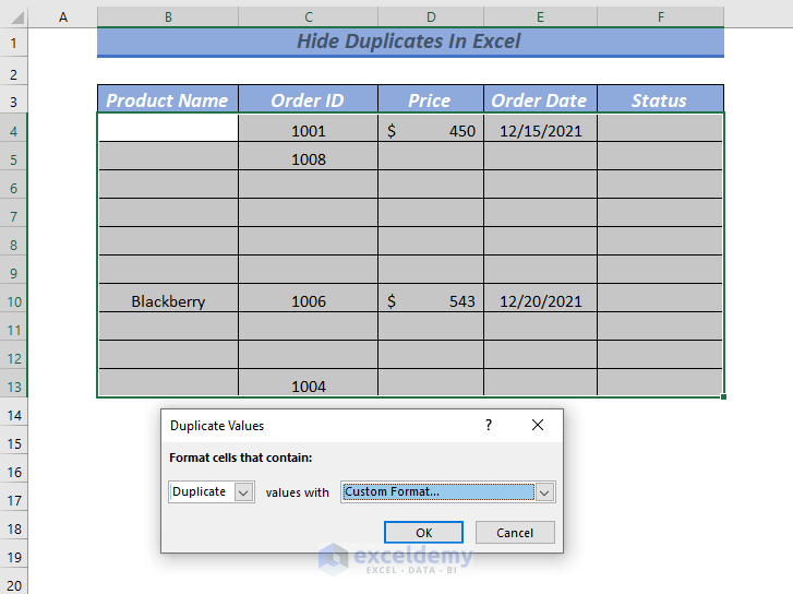
As a result, all duplicate values, including the first occurrence, will be hidden in your dataset.
Read More: Excel Remove Duplicates Not Working
Method 4 – Hide Duplicates Using Formula in Condition Formatting
You can utilize any formula in Conditional Formatting to format cells or cell ranges. In this method, we’ll apply a formula to hide duplicates in the dataset.
- Select the cell range where you want to apply the formula for formatting. For example, choose the cell range B4:F13.
- Follow these steps:
- Open the Home tab.
- Under Conditional Formatting, select New Rule.
- A dialog box will appear.
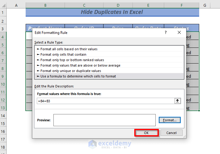
- In the dialog box:
- Choose Use a formula to determine which cells to format under Select a Rule Type.
=B4=B3-
-
- This formula checks if the value in the active cell (B4) is equal to the cell above it (B3). If they are equal, the result of this formula is TRUE, and formatting will be applied to the cells; otherwise, if they are not equal, the result is FALSE, and no format will be applied.
-
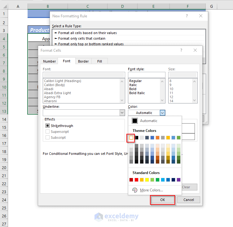
- Click on Format to choose the format.
- Another dialog box will pop up for selecting the format.
- In the second dialog box, you can select any color. However, to hide duplicates, choose a color that matches the background of your cell.
- For example, if your cell color is White, select White as the format color.
- Click OK on the Edit Formatting Rule dialog box.
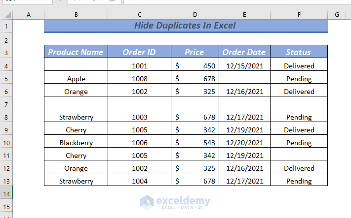
As a result, all consecutive duplicate values will be hidden in your dataset.
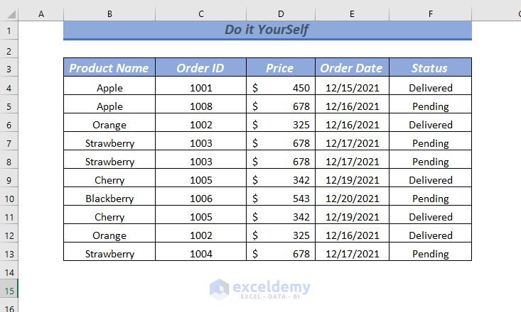
Practice Section
A practice sheet has been provided in the workbook to practice these explained examples.
Download to Practice
You can download the practice workbook from here:
Further Readings
- How to Remove Duplicate Names in Excel
- Remove Both Duplicates in Excel
- How to Remove Duplicate Rows in Excel Table
- How to Remove Duplicates but Keep the First Value in Excel
- Remove Duplicate Rows Except for 1st Occurrence in Excel
- How to Delete Duplicates But Keep One Value in Excel
- How to Undo Remove Duplicates in Excel
<< Go Back to Remove Duplicates in Excel | Learn Excel
Get FREE Advanced Excel Exercises with Solutions!
