Project Cost Estimation Example in Excel (with Easy Steps)

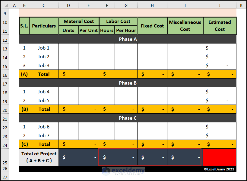
Step 1 – Create Basic Outline

This should be divided into two different parts. One is the short information about the project and the other is the cost calculation part.

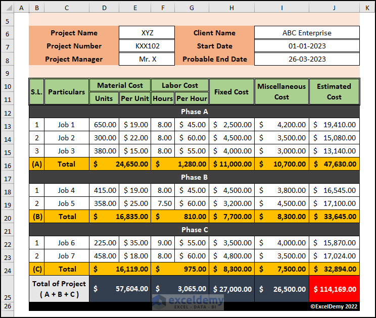
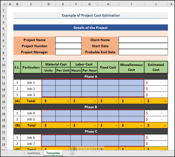
• In the info area, we included the Project Name, Project Number, Project Manager, Client Name, Start and End Date of the Project in the B6:J8 range.

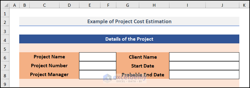
• In the cost calculation part, we created a table to contain different cost components and their amount. We’ll calculate these amounts step-by-step in the following part of the article.

Read More: How to Perform Building Estimation and Costing in Excel Sheet

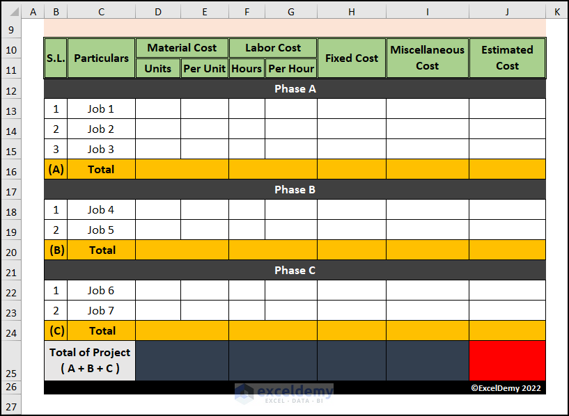
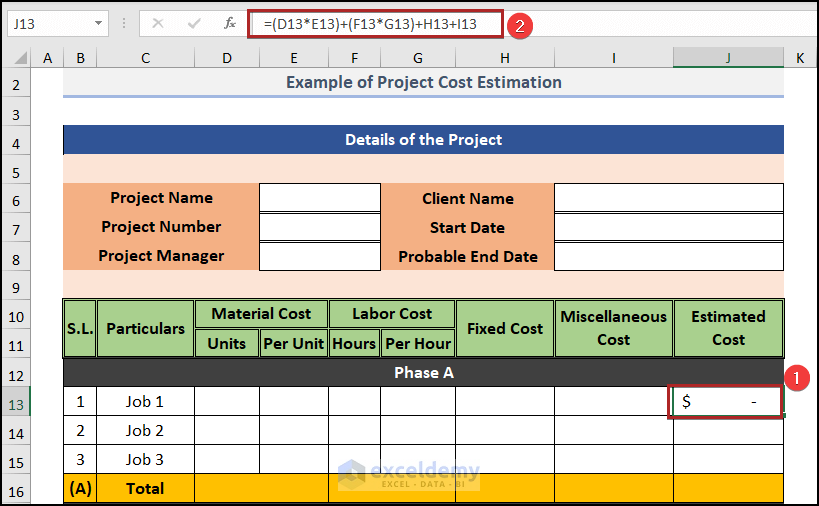
Step 2 – Estimate Phase-wise Total Cost

• Go to cell J13 and enter the following formula:

Here, D13 and E13 represent the Units and Per Unit cost of Material. Also, F13 and G13 serve as the Hours and Per Hour cost of Labor. On the other hand, H13 and I13 substitute the Fixed Cost and Miscellaneous Cost.

• Press Enter.

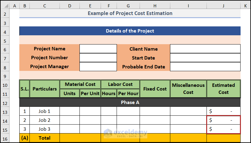
•  Drag the formula down to the other cells in the column.

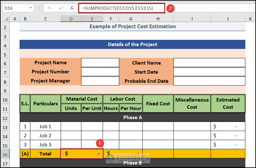
• Go to cell D16 and insert the formula below.

Here, we used the SUMPRODUCT function to take two arrays (D13:D15 and E13:E15) as arguments, multiply the corresponding values of all the arrays, and then return the sum of the products.

• Press Enter.

• Use the same formula to calculate the Total Labor Cost.
• SUM the cells in the columns to the Total Fixed Cost and the Total Miscellaneous Cost of this phase.
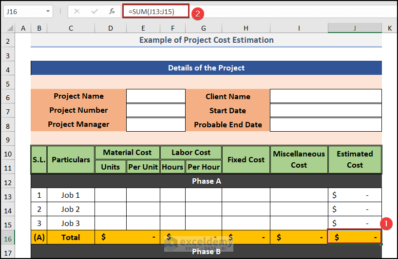
• Select cell J16 and write down the formula below.

• Press Enter.

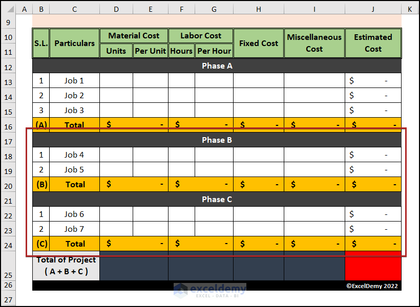
• You can calculate them for Phase B and C as well.

Read More: How to Calculate Residential Construction Cost Estimator in Excel

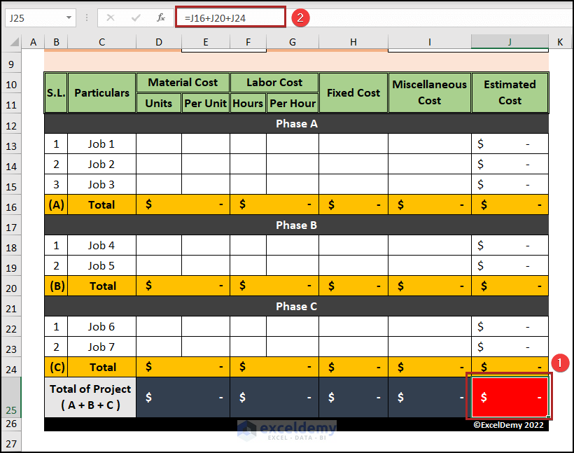
Step 3 – Calculate Total Estimated Project Cost

• Select cell D25 and paste the following formula.

• Press Enter.

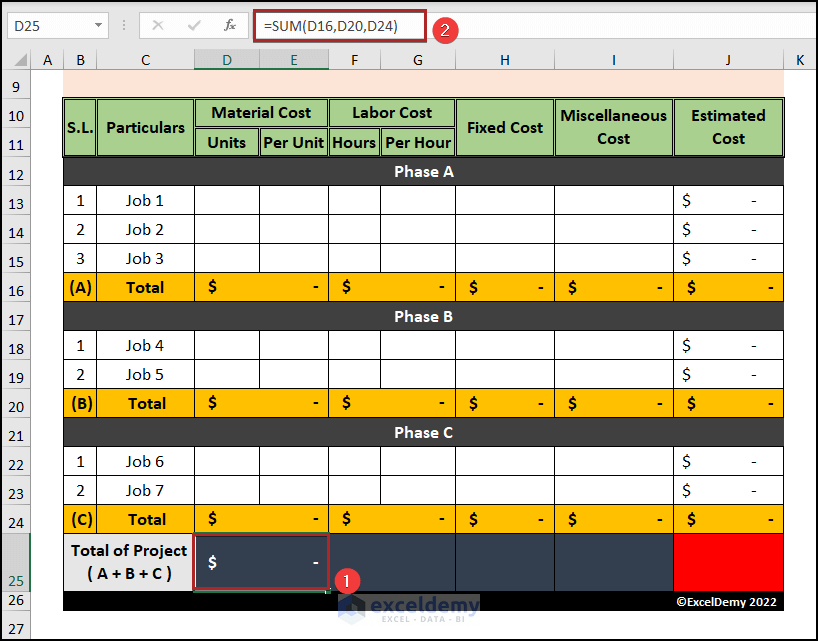
• Do the same for Labor, Fixed, and Miscellaneous costs.

• Select cell J25 and put down the formula below.

• Hit Enter.

Read More: How to Make an Effort Estimation Sheet in Excel 

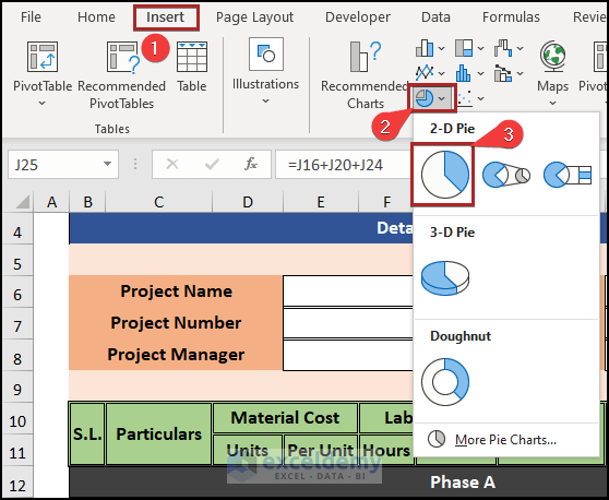
Step 4 – Insert a Chart to Aid in Visualization

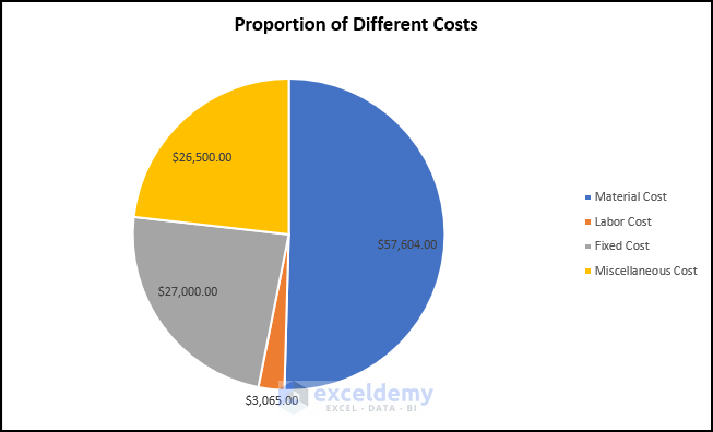
• Navigate to the Insert tab.
• Click on the Insert Pie or Doughnut Chart drop-down icon.
• Select the Pie chart from the 2-D Pie section.

• Change the chart title and give a suitable one.

• Right-click anywhere inside the chart area to open the context menu.
• Click on the Select Data… option.

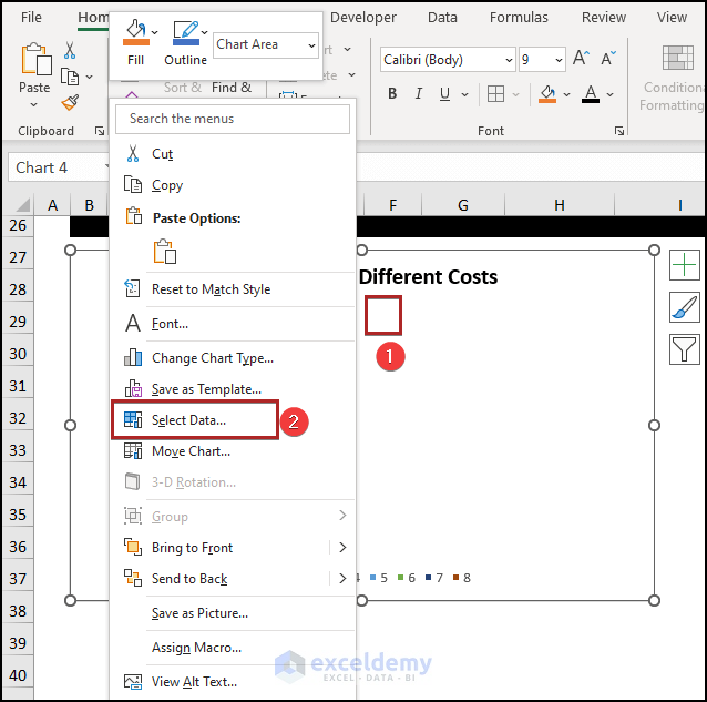
• In the Select Data Source dialog box, tap on the Edit button under the Horizontal (Category) Axis Labels section.

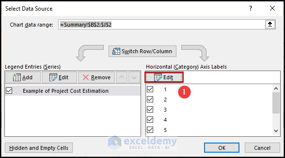
As axis labels, we want to show the different cost components like material cost, labor cost, etc.

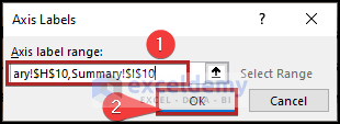
• In the Axis Labels dialog box, select those cells (D10, F10, H10, and I10) to get the value in the Axis label range box.
• Click OK.

• Click OK.

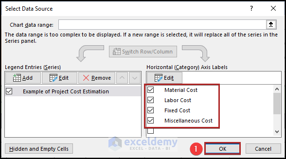
• Bring the Select Data Source box.
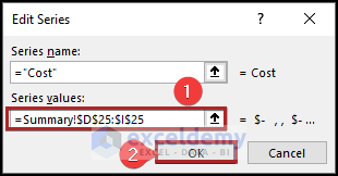
• We renamed the series as Cost. Select it and click on the Edit button.

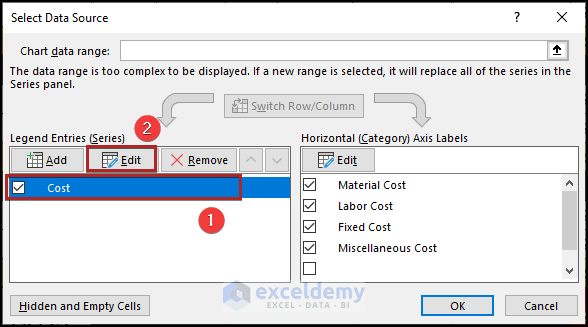
Instantly, the Edit Series box will pop up.

• Give the cell references of the total amount of different cost components. For example, D25 has the total material cost, and F25 has the total labor cost.
• Click OK.

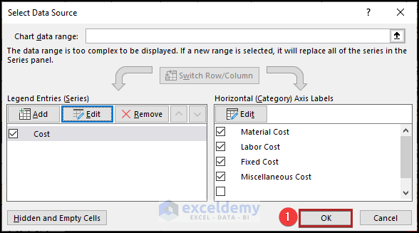
• Click on the OK button.

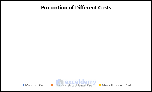
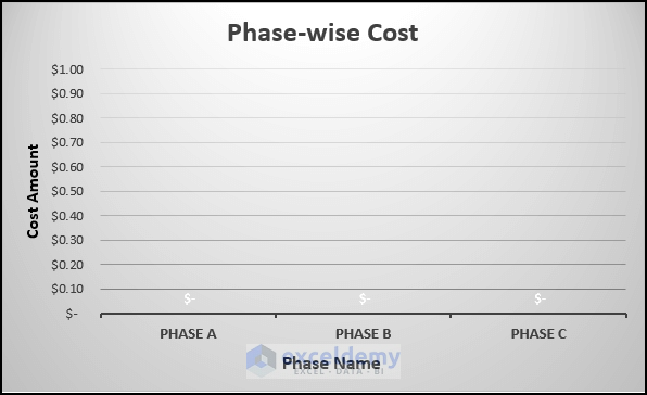
We can see a blank chart like the following.

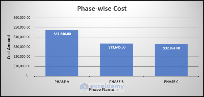
Similarly, we inserted another Column Chart to plot the phase-wise cost of the project.

Step 5 – Verify with Sample Data

• We inserted sample data in the blank cells and the results are before our eyes.

The charts are in the following states now.

Read More: How to Do Interior Estimation in Excel

Free Template of Project Cost Estimation [Ready to Use]

You can use the template instantly by just downloading the Excel file. Write down your values in the light-blue-colored cells.

Read More: How to Make House Estimate Format in Excel

Things to Remember

#N/A! error arises when the formula or a function in the formula fails to find the referenced data.

#DIV/0! error happens when a value is divided by zero (0) or the cell reference is blank.

Download Practice Workbook

You may download the following Excel workbook for better understanding and practice.