How to Create a Route Map in Excel (Two Methods)

Method 1 – Utilizing Google Maps

In this approach, we will explore creating a route map using Microsoft Excel and Google Maps.

Steps

Prepare Your Data:
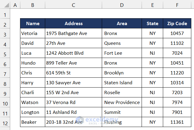
- Begin with a dataset containing information about the locations you want to include in your route map. For our example, we’ll use a dataset of 10 people.
- The names of these individuals are listed in column B, and their detailed address information is spread across columns C, D, E, and F.

Save Your Data as a CSV File:
- Open your Excel file.
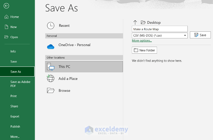
- Click on the File tab, then select Save As.
- In the Save A” window, choose a suitable name for your file (e.g., Make a Route Map).
- Change the file format to CSV (MS-DOS) (*.csv).

Check the CSV File in Notepad:
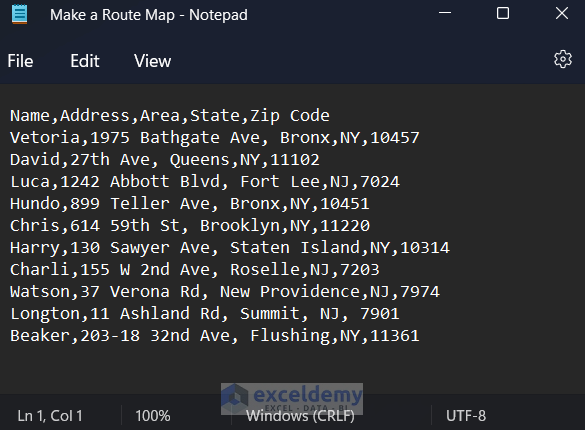
- Right-click on the saved CSV file and open it in Notepad.
- Verify that the information is formatted correctly according to your requirements.

Create a New Map Using Google My Maps:
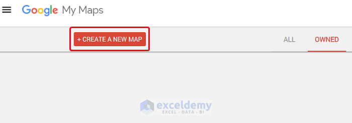
- Open a web browser and search for Google My Maps.
- Click on the Create A New Map option.

- Rename the map according to your preference (e.g., Make Route Map).

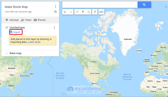
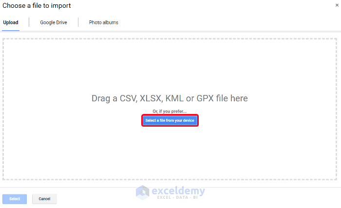
Import Your CSV File:
- Select Import and then choose Select a file from your device.

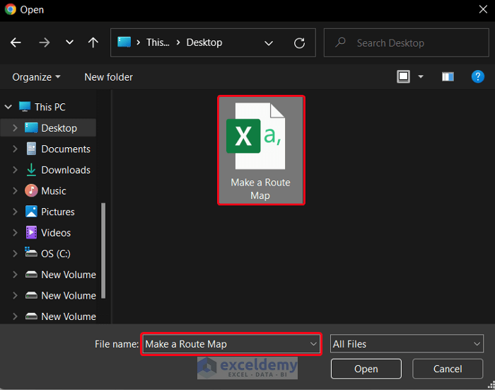
- In the dialog box that appears, locate and open your Make a Route Map.csv file.

- Wait for the file to load into the website.

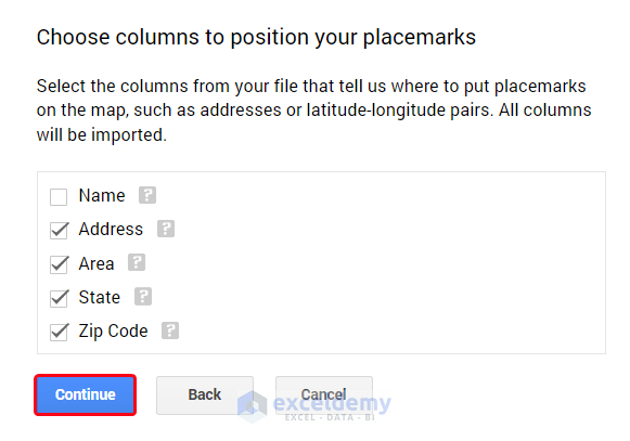
Position the Placemarks:
- A small window will appear, asking you to choose the columns to position the placemarks. Select all columns except for the Name column.
- Click Continue.

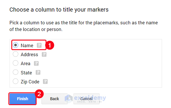
Set Marker Titles:
- Another window will prompt you to choose the title for your markers. Select the Name column as the marker title.
- Click Finish.

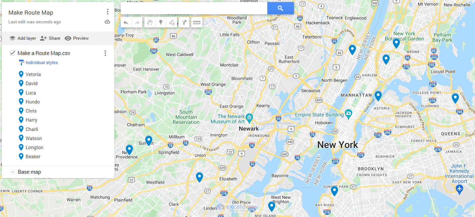
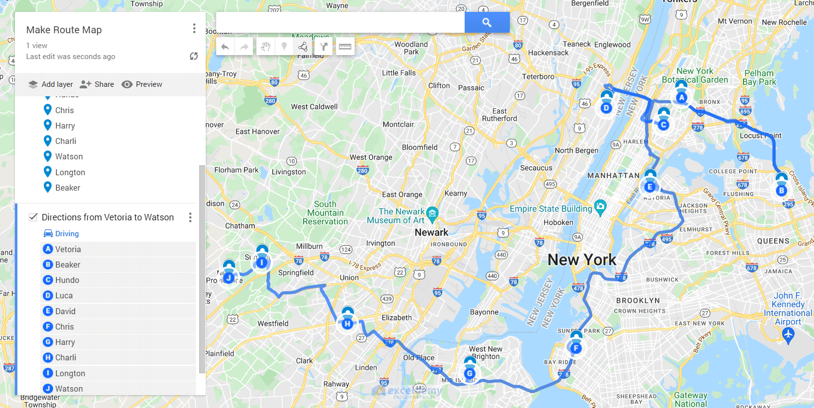
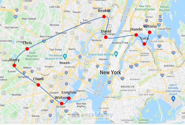
Trace Locations on the Map:
- After a brief processing time, you’ll see all the locations traced on the map.

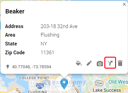
Add Directions:
- Click on the marker (represented by a beaker icon) and select the Direction to here option.

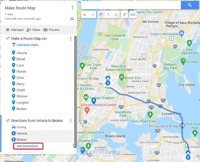
- A new layer called Route will be added below the current layer.

- Select the second place in your route.

- Click Add Destination and add subsequent spots to complete the route.

Completion:
- Congratulations! Your route map is now complete.
- This method allows you to create a route map directly within Excel using Google Maps.

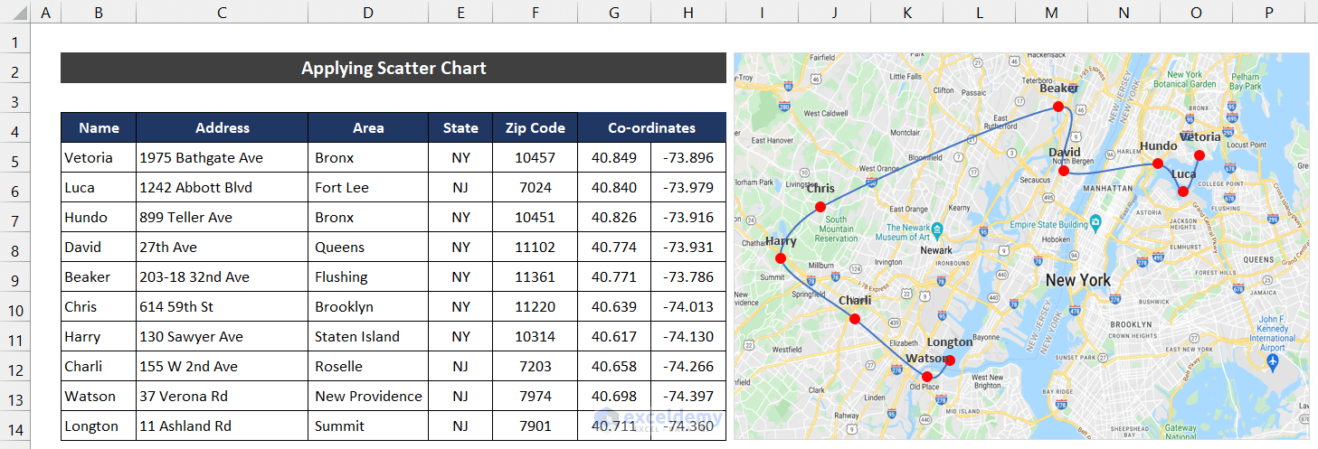
Method 2 – Creating a Route Map with a Scatter Chart

In this method, we’ll use a scatter chart to create a route map in Excel. Unlike the previous approach, we’ll work with coordinates to represent locations. Follow the steps below:

Gather Coordinates:
- Obtain the coordinates for each location. You can find these coordinates from our previous map or by searching directly on Google Maps.

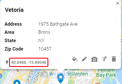
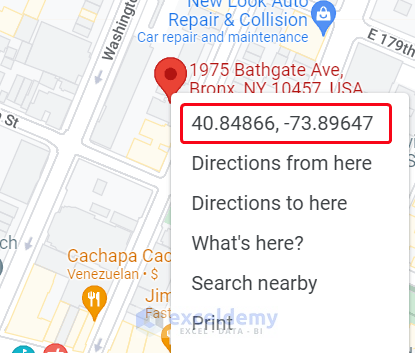
- Right-click on a marker to view its coordinates at the top of the list.
- Copy the coordinate value.

Paste Coordinates into Excel:
- Paste the copied coordinate values into an Excel worksheet (use Ctrl+V).
- Repeat this process for all the coordinates.

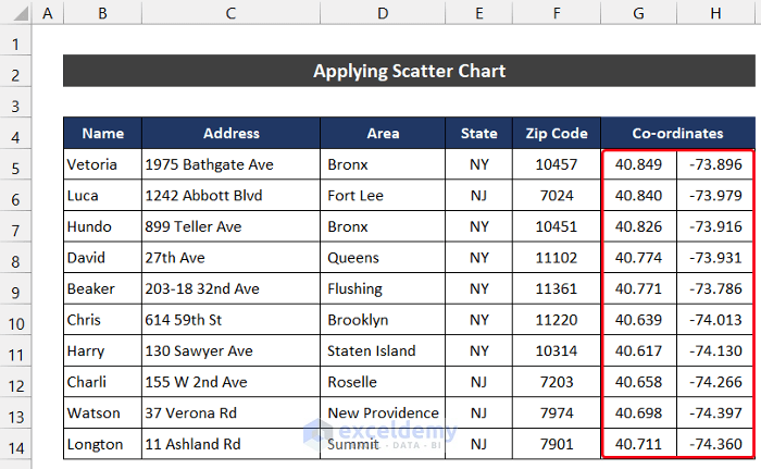
Select the Data Range:
- Highlight the range of cells containing the coordinates (e.g., G5:H14).

Create a Scatter Chart:
- Go to the Insert tab.
- Click the dropdown arrow next to Scatter (X, Y) or Bubble Chart and choose Scatter with Smooth Lines and Markers from the Charts group.

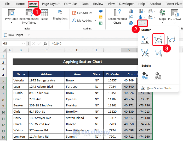
- The scatter chart will appear.

Customize Data Labels:
- Remove unnecessary chart elements, leaving only the data labels.

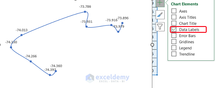
- Double-click on any data label to open the Format Data Labels side window.
- Under Label Options, uncheck all options except Value From Cells.
- Specify the range of cells (B5:B14) containing the corresponding person’s names.

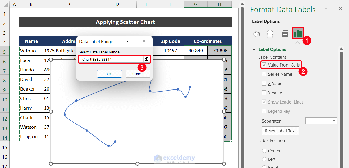
You will see all the points got the corresponding person’s name.

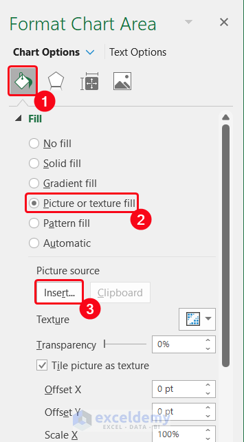
Enhance the Chart:
- To make the chart more meaningful, select it and go to Fill & Line options.
- Choose Picture or Texture Fill.
- Insert an image of the map that covers the area of interest, making the chart resemble a real map.

Customize Points:
- Modify the appearance of the blue points on the chart according to your preference.

Completion:
- Congratulations! Your route map is now ready.

Things You Should Know

Keep in mind that this method relies on an image of the map, so the scale may not match the actual geography precisely.
Use this chart as a prediction tool for understanding a person’s location and their neighbors, but exercise caution and verify information when needed.

Download Practice Workbook

You can download the practice workbook from here:

Make a Route Map.xlsx

Make a Route Map.csv