How to Make Excel Move Automatically to the Next Cell (4 Suitable Ways)

Looking for ways to know how to make Excel move automatically to the next cell? Sometimes, we want our Excel to move to the next cell automatically to make our work easier. Here, you will find 4 different step-by-step explained ways to make Excel move automatically to the next cell.

How to Make Excel Move Automatically to Next Cell: 4 Ways

We can make Excel move automatically to the next cell by using the following 4 step-by-step ways.

1. Using VBA to Make Excel Move Automatically to Next Cell

Here, we have a dataset containing the values of User Name of some students on a website. In the User Name, the first 5 letters are their Name and the rest of the 5 letters are their Roll numbers.

Now, we will use VBA to automatically move the letters to the next cells.

Follow the steps below to do it on your own.

Steps:

First, go to the Developer tab >> click on Visual Basic.

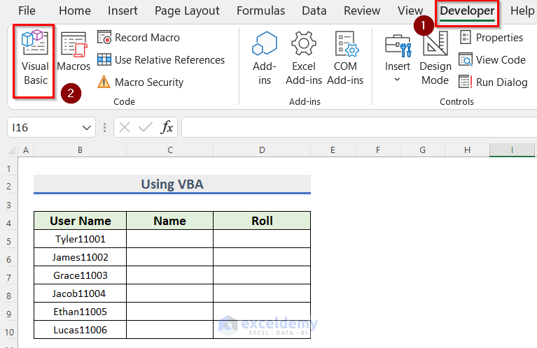
Now, the Microsoft Visual Basic for Applications will open.
Then, go to the Insert tab >> select Module.

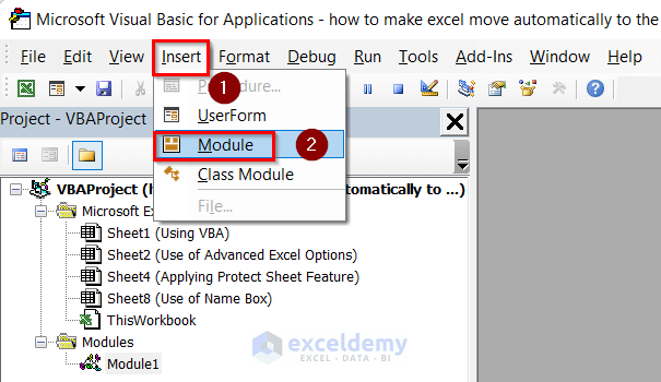
Then, write the following code in your Module.

Sub Move_to_Next_Cell()
Dim Str As String
Dim start_position As Integer
Dim column_number As Integer
Str = Application.InputBox("Enter value", "Move to Next Cell", , , , , , 2)
column_number = 0
Application.ScreenUpdating = False
For start_position = 1 To Len(Str) Step 5
    ActiveCell.Offset(0, column_number) = "'" & Mid(Str, start_position, 5)
    column_number = column_number + 1
Next
Application.ScreenUpdating = True
End Sub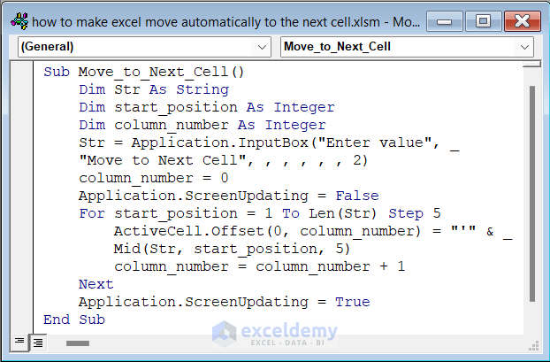

Code Breakdown

First, we created a Sub Procedure as Move_to_Next_Cell.
Then, we declared Str as String, start_position and column_number as Integer.
After that, we set InputBox named as Move to Next Cell to Enter Value.
Next, we selected column_number=0
Afterward, we set the Screen Updating to False.
Then, we used a For loop from start_position = 1 to the length of the Str and set Step as 5.
Now, we used the VBA Mid function to extract the first 5 character and by using the VBA Offset function moved the extracted values to the next cell.
After that, incremented the column_Number by using column_Number = column_Number+ 1.
Next, we set the Screen Updating as True.

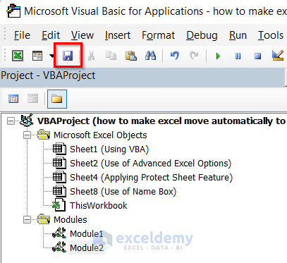
Next, click on the Save button and go back to your worksheet.

Now, select the Cell C5.
After that, go to the Developer tab >> click on Macros.

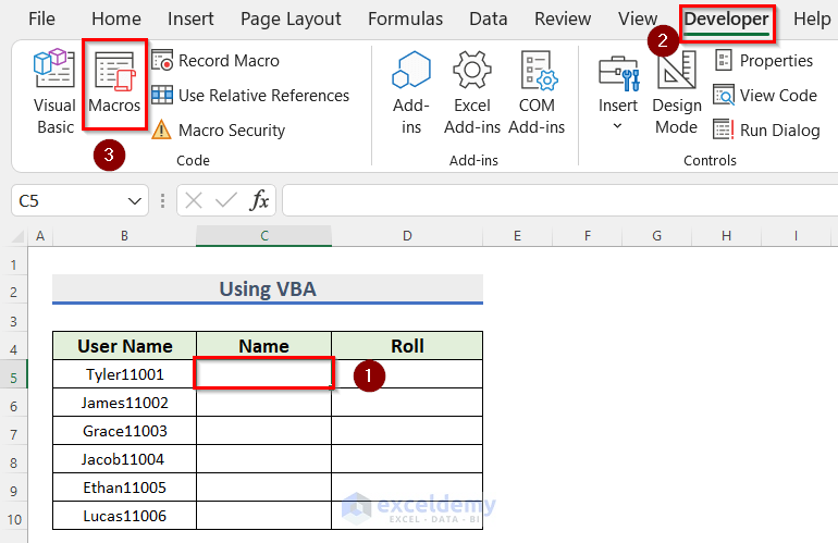
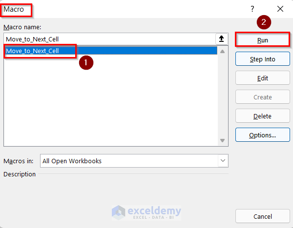
Now, the Macros box will appear.
Then, select Move_to_Next_Cell macro.
After that, click on Run.

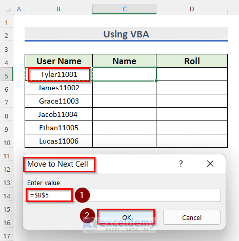
Next, the Move to Next Cell box will open.
Then, in the Enter value box select Cell B5.
After that, click on OK.

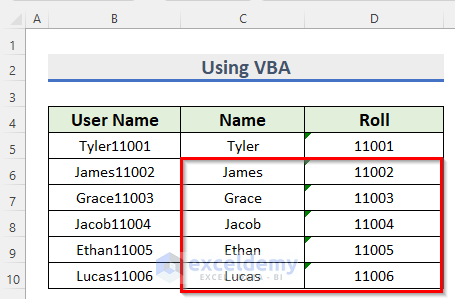
Now, you can see that the Cell value of B5 has moved to Cell C5 and Cell D5. Cells C5 contains the first 5 letters and Cell D5 contains the rest of the 5 letters.

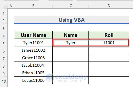
Finally, follow the same steps we have done for Cell D5, for the rest of the cells to move Excel automatically to the next cell.

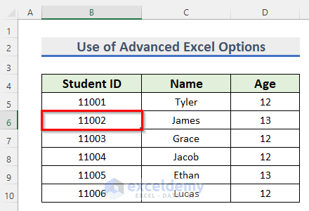
2. Use of Advanced Feature from Excel Options to Move Automatically to Next Cell

Sometimes when we click on the ENTER Excel does not move to the next Cell. Here, we will use Advanced Excel Options to move automatically to the next cell in Excel.

Steps:

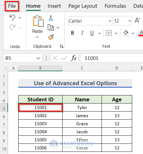
First, select and click on Cell B5.
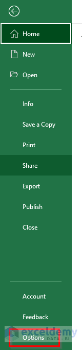
Then, go to the File tab.

After that, click on Options.

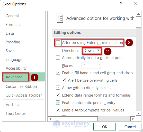
Now, the Excel Options box will open.
Next, go to the Advanced option.
Then, turn on the After pressing Enter, move selection and set Direction as Down.
After that, press OK.

Finally, click ENTER.
Now, you can see that Cell B5 has moved downward to Cell B6.

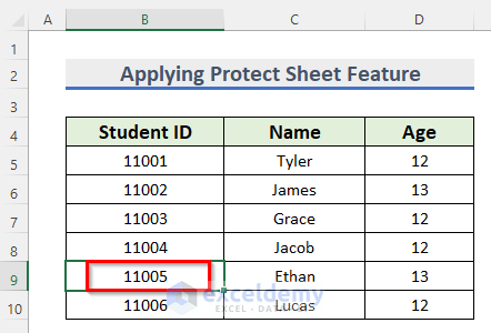
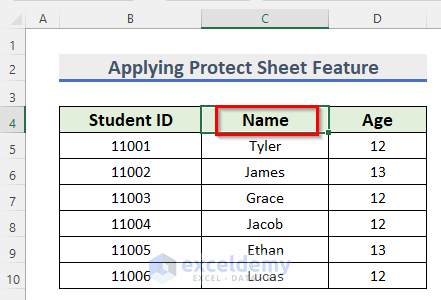
3. Applying Protect Sheet Feature to Move Automatically to Next Cell

Now, we will apply the Protect Sheet Feature to move Excel automatically to the next cell.

Go through the steps given below to do it on your own.

Steps:

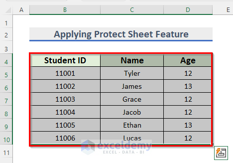
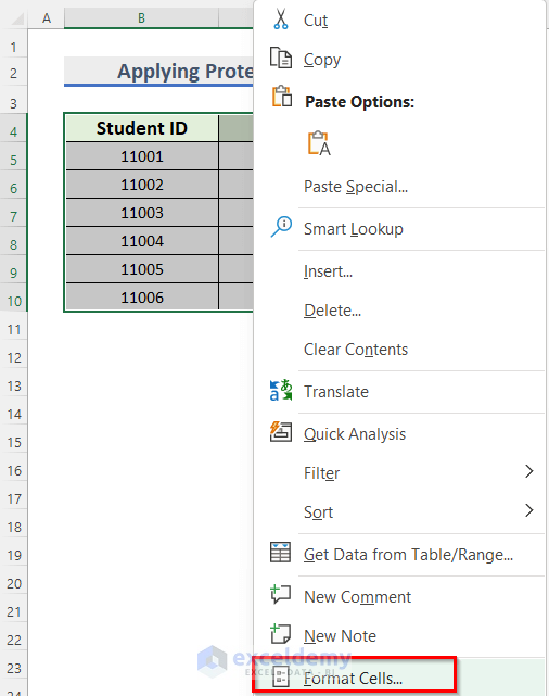
First, select the Cell range B4:D10 and right-click.

Then, click on Format Cells.

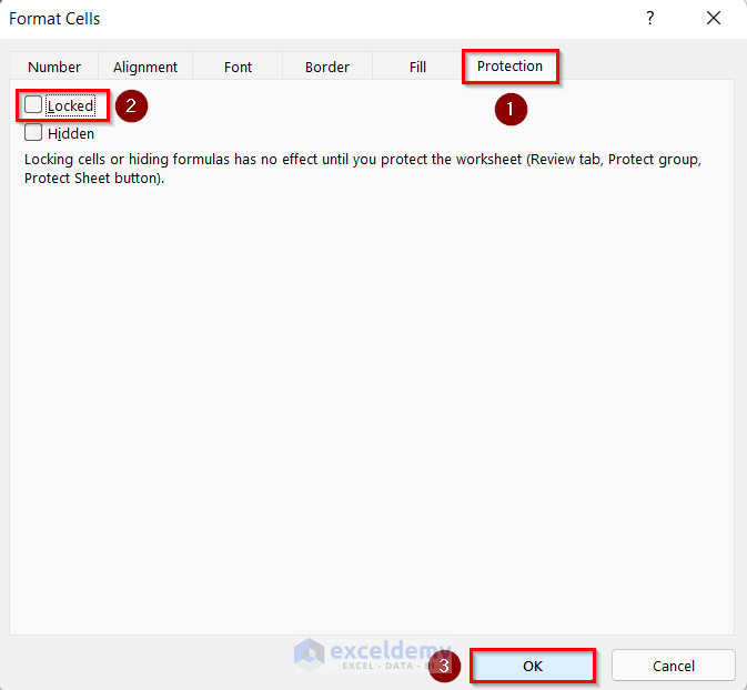
Now, the Format Cells box will appear.
Next, go to the Protection tab.
After that, unselect the Locked option.
Then, click on OK.

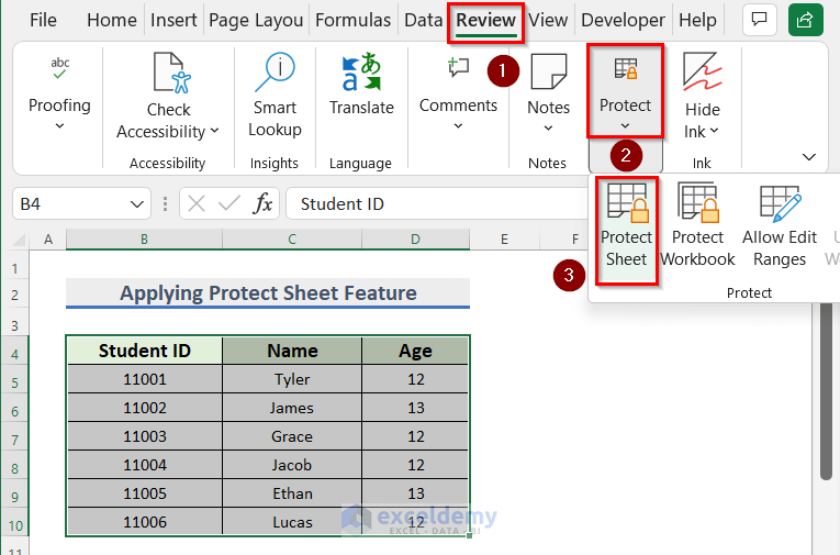
Next, go to the Review tab >> click on Protect >> select Protect Sheet.

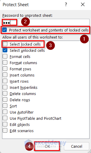
Now, the Protect Sheet box will open.
After that, turn on the Protect worksheet and contents of locked cells.
Then, set a Password. Here, we set “123” as a Password.
Next, unselect the Select locked cells option.
Afterward, click on OK.

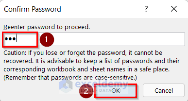
Then, to confirm the Password type the Password again in the box.
Next, click on OK.

Now, click on Cell B10.

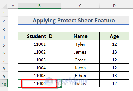
Next, press ENTER.
Here, you can see that Cell B10 has moved to Cell C4 rather than Cell B11 as the Cell range has been locked using the Protect Sheet Feature.

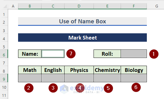
4. Use of Name Box to Make Excel Move Automatically to Next Specific Cell

In the final method, we will show you how to make Excel move automatically to the next specific Cell using the Name Box.

Here, we have a dataset where we have to insert the Name, Roll, and Marks in Math, English, Physics, Chemistry, and Biology of a student in their Specific Cells.

Steps:

First, select Cell F6.
Then, press CTRL and select Cell B9, C9, D9, E9, F9, and C6 respectively.

After that, click on the Name box.
Next, type Marks.
Then, press ENTER.

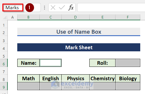
Now, you can see that Cell C6 is selected.
Next, insert any Name of your own preference. Here, we will insert “Lucas”.

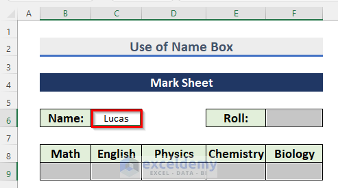
Afterward, press ENTER.
Then, Cell C6 will move to Cell F6.
Next, insert “12001” as Roll.

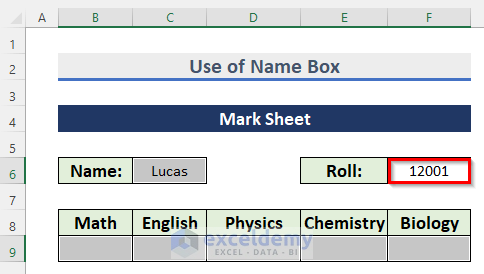
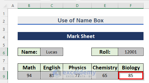
Now, if you press ENTER the Cells will move to Cell B9, C9, D9, E9, and F9 respectively, and insert the data according to your preference.

Here, we inserted 94, 81, 77, 65, and 85 in Cell B9, C9, D9, E9, and F9 respectively.

Practice Section

In this section, we are giving you the dataset to practice on your own and learn to use these methods.

Download Practice Workbook

Automatically Move to Next Cell.xlsm

Conclusion

So, in this article, you will find 4 ways to make Excel move automatically to the next cell. Use any of these ways to accomplish the result in this regard. Hope you find this article helpful and informative. Feel free to comment if something seems difficult to understand. Let us know any other approaches which we might have missed here.

<< Go Back to Move Cells | Excel Cells | Learn Excel

Get FREE Advanced Excel Exercises with Solutions!

2 Comments

Ole Dagfinn Tandberg Oct 12, 2023 at 5:47 PM

I have two Excel sheets:

Startlist: With bib number and starttime and names

Results: I using VBA to lookup bib numbers from startlist and then calculate finish time

Problem: RFID reader put in bib number but i need to push enter key so Excel is ready for next value from RDID reader. I want Excel to automaticly move to next cell under after RFID value is set by RFIS reader

Regards
Ole Dagfinn Tandberg
- Reply
  Seemanto Saha Oct 16, 2023 at 10:48 AM
  Hello OLE DAGFINN TANDBERG,
  Thanks for sharing your problem with us. I understand that you are facing problems with automatic value entry from the RFID reader.
  
  Usually, an RFID reader places values (e.g. bib number, name, start time, finish time, etc.) in cells of newer rows automatically by moving one row down. That means if the first RFID reading places values in Row 1, then the second RFID reading should automatically place values in ROW 2, the third RFID reading should automatically place values in ROW 3, and so on.
  
  But in your case, you have to press the Enter key to move one row down. This is probably due to the RFID reader or software configuration. It is possible that the RFID reader software places values in cells of Active Row (i.e. the row of Active Cell) but does not offset the active cell by 1 row down for the next set of entries.
  
  The best solution to this problem is to modify the settings of the RFID reader. If that is not possible, you can use a VBA code to change the Active Row each time an RFID reading is performed.
  
  Right-click over the Sheet Tab of the Startlist sheet and select the View Code option.
  
  At this point, the Visual Basic Editor for that sheet will open. Insert the following code in the editor module.
  
  Excel VBA Code
```
Private Sub Worksheet_Change(ByVal Target As Range)
    Dim activeRowChange_column As String
    activeRowChange_column = "C" ' change this according to your requirement
    
    Set activeRowChange_range = ThisWorkbook.ActiveSheet. _
    Range(activeRowChange_column & ":" & activeRowChange_column)
    
    If Not Intersect(Target, activeRowChange_range) Is Nothing Then
        Target.Offset(1, -2).Select
    End If
End Sub
```
  As your Startlist sheet would have 3 values (i.e. bib number, start time, and name), I have assumed that the cell from the Active Row of Column C will be the last cell updated from an RFID reading. When a cell in Column C is updated from the RFID reading, the active row will automatically move to the next row and be ready for the next RFID reading value entry.
  
  Repeat the same steps for the “Results” sheet as well.
  
  To demonstrate this actually works, we will use a User Form to enter values in the Startlist and Results sheets.
  
  After entering the Bib Number and Name, when we click the Submit button (similar to scanning a card in the RFID reader), the Bib Number, Starting Time, and Name will be saved in the Active Row of the Startlist sheet. As soon as these records are saved, the active row will automatically move to the row below. You can notice this in the following GIF:
  
  Now, If you enter another Bib Number and name, and click the Submit button it will be saved in a new row. You can watch this in the following GIF:
  
  On the other hand, if you reenter the Bib Number and Name, and click the Submit button, it will look up the Bib Number in the Startlist sheet, calculate Final Time, and insert the Bib Number, Final Time, and Required Time in the Results sheet. As soon as these values are saved, the active row will move to the row below automatically. You can watch that in the following GIF:
  
  As the User Form was used only to demonstrate how the Active Row moves one row below, we haven’t included the code used in the User Form. But you can find the codes in the following workbook.
  
  WORKBOOK
  
  Hopefully, this solution will be helpful for you. However, as we have assumed a lot of properties of your Workbook and the RFID reader, this solution can vary from the actual required solution. Please share your workbook and the working process of the RFID reader in such an instance.
  
  Regards,
  Seemanto Saha
  ExcelDemy

How to Make Excel Move Automatically to the Next Cell (4 Suitable Ways)

How to Make Excel Move Automatically to Next Cell: 4 Ways

1. Using VBA to Make Excel Move Automatically to Next Cell

2. Use of Advanced Feature from Excel Options to Move Automatically to Next Cell

3. Applying Protect Sheet Feature to Move Automatically to Next Cell

4. Use of Name Box to Make Excel Move Automatically to Next Specific Cell

Practice Section

Conclusion

Related Articles

Leave a reply Cancel reply