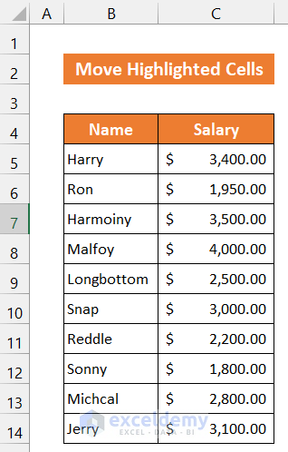
How to Move Highlighted Cells in Excel (5 Ways)

We’ll use the data of 10 employees of a company. Their names and salaries are in columns B and C. We will highlight the entities that are in the Salary range between $3,000 and $4,000. Then, we will move them to the top or bottom of our dataset.

Method 1 – Use the Sort Command to Move Highlighted Cells

Steps:

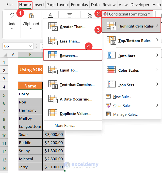
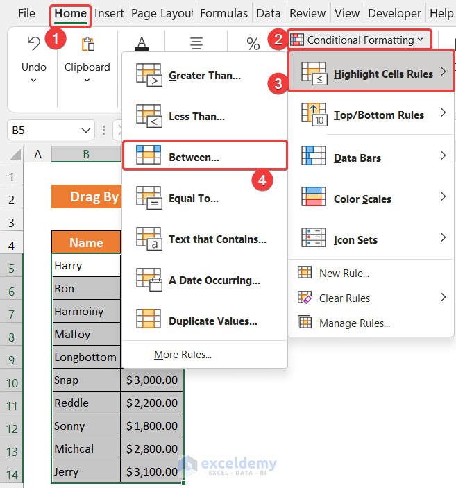
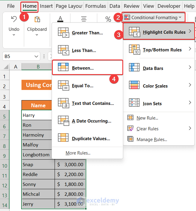
Select the entire range of cells B4:C14.
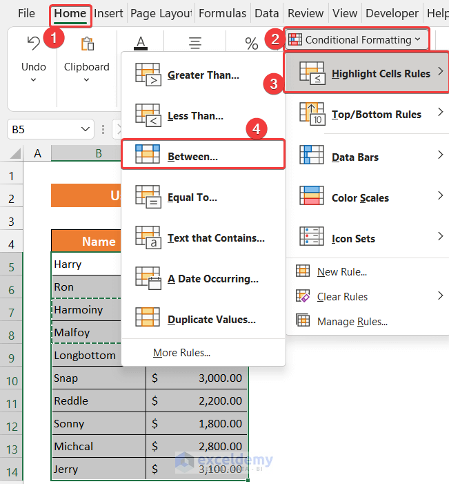
In the Home tab, select Conditional Formatting.
Click on Highlight Cell Rules and choose Between.

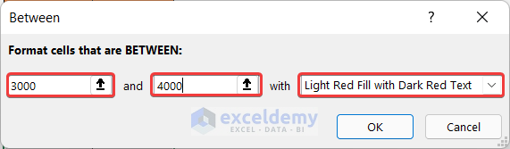
A small dialog box called Between will appear.
Write down your desired lowest and highest salary amount like the image shown below. We choose the salary range of $3,000 to $4,000.
Choose the cell highlight pattern. We kept the default one, Light Red Fill with Dark Red Text.

Click OK to close the dialog box.

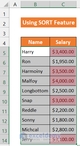
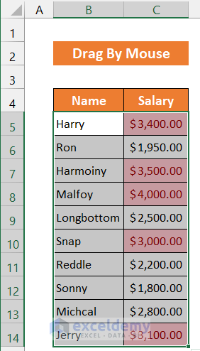
You will see the salaries within the range highlighted.
In the Data tab, select the Sort & Filter group.
Click on Sort.

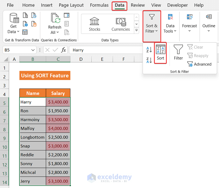
A small dialog box called Sort will appear.
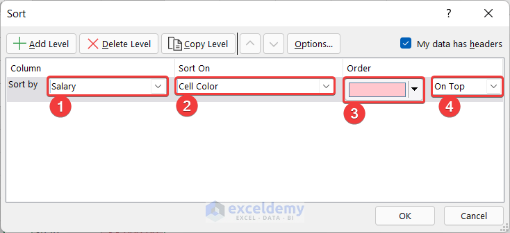
Click on the drop-down arrow of the Column option and choose Salary.
Change the Sort On option from Cell Values to Cell Color.
Click on the drop-down arrow of the Order option and choose the cell color.
Next to the Order drop-down, there is another drop-down. Click on it and you will get 2 options. On Top/On Bottom. Choose one. We kept the On Top option.
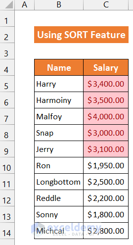
Click OK.

You will find all the highlighted rows move up.

Things You Should Know

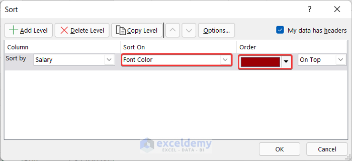
As our highlight pattern contains both the cell color and font color, you can also choose the Sort On option with Font Color. The result of both selections will be the same.

Method 2 – Drag the Highlighted Cells to Move

Steps:

Select the entire range of cells B4:C14.
In the Home tab, select Conditional Formatting.
Click on Highlight Cell Rules and select Between.

A small dialog box called Between will appear.
Write down your desired lowest and highest salary amount like the image shown below. We chose the salary range of $3,000 to $4,000.
Choose the cell highlight pattern. We kept the default one, Light Red Fill with Dark Red Text.
Click OK to close the dialog box.

You will see the salaries within the range highlighted.

Select any of those highlighted cells with your mouse.
If you hover over the edge of the cell, a Move Pointer icon will appear.

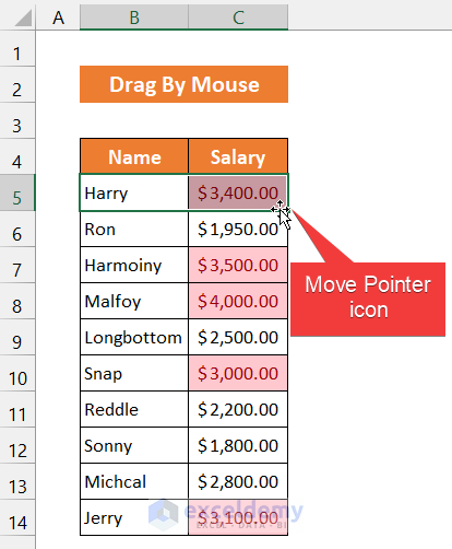
Select the Move Pointer icon and drag it to the bottom of the dataset with your mouse.

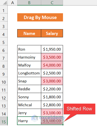
Repeat for all of the highlighted cells.
When you drag the rows through your mouse, an empty row will be created at that position. Select all of those empty rows.

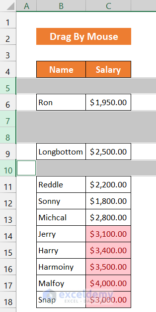
In the Home tab, go to the Cells group and click Delete.

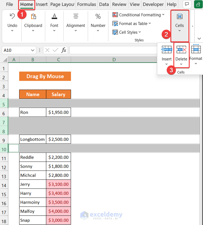
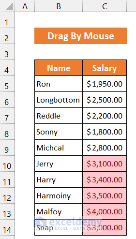
You will get all the highlighted cells at the bottom of your dataset.

Method 3 – Move the Highlighted Cells Using the Insert Option

Steps:

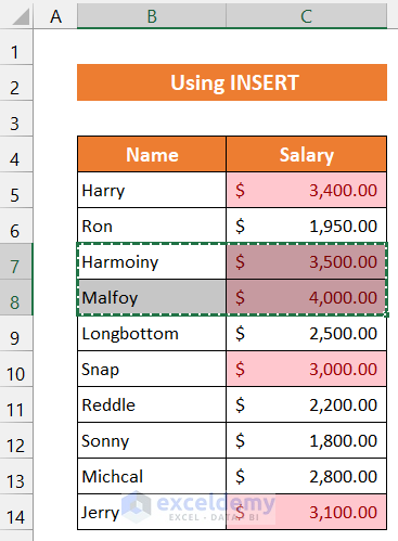
Select the entire range of cells B4:C14.
In the Home tab, select Conditional Formatting.
Click on Highlight Cell Rules and choose Between.

A small dialog box called Between will appear.
Write down your desired lowest and highest salary amount like the image shown below. Here, we choose the salary range of $3,000 to $4,000.
Choose the cell highlight pattern. We kept the default one, Light Red Fill with Dark Red Text.
Click OK to close the dialog box.

You will see the salaries within the range highlighted.
Select the range of cells B7:C8.
Press Ctrl + X on your keyboard.

Select cell B6 and, in the Home tab, select Insert from the Cells group.

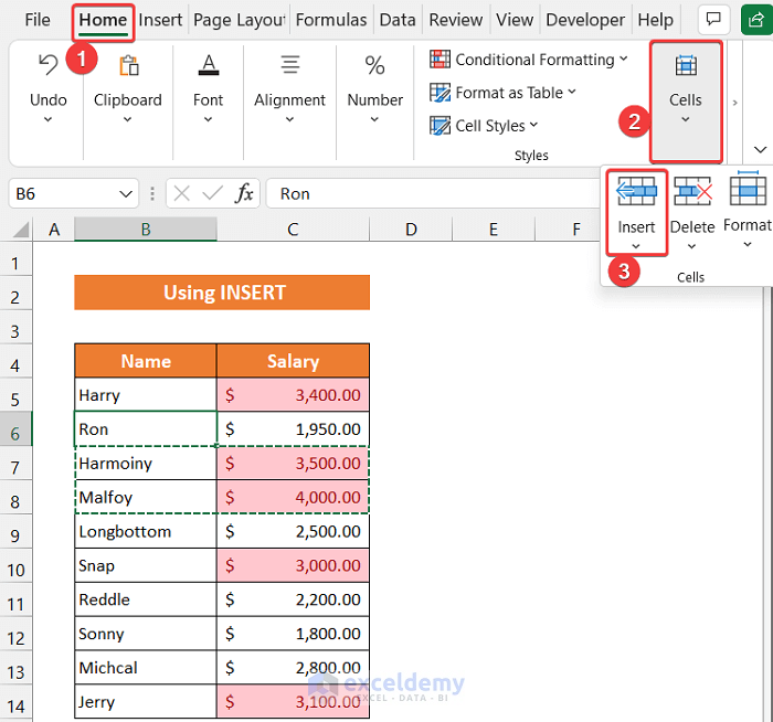
The range of the cells will move upward.

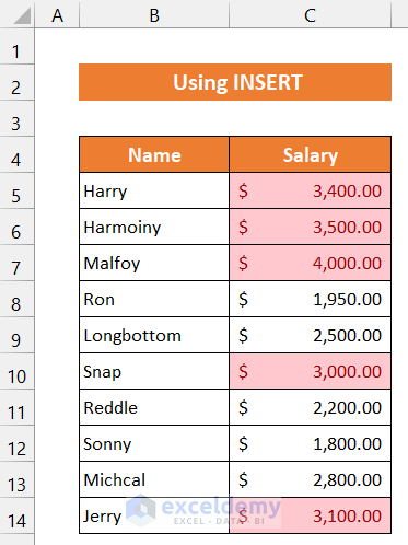
Follow the same procedure for the rest range of cells B10:C10 and B14:C14.
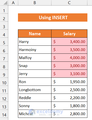
You will get all the highlighted cells at the top of your dataset.

Method 4 – Using the Shift Key to Move Cells

Steps:

Select the entire range of cells B4:C14.
In the Home tab, select Conditional Formatting.
Click on Highlight Cell Rules and choose Between.

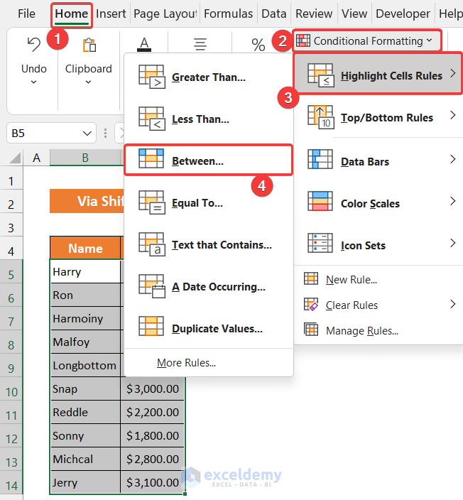
A small dialog box called Between will appear.
Write down your desired lowest and highest salary amount like the image shown below. We chose the salary range of $3,000 to $4,000.
Choose the cell highlight pattern. We left the default one, Light Red Fill with Dark Red Text.
Click OK to close the dialog box.

You will see the salaries within the range highlighted.
Select the range of cells B7:C8.
Press the Shift key and drag the Move Pointer.

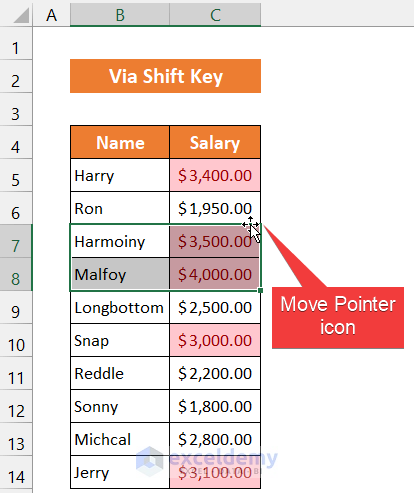
The range of cells will move upward.

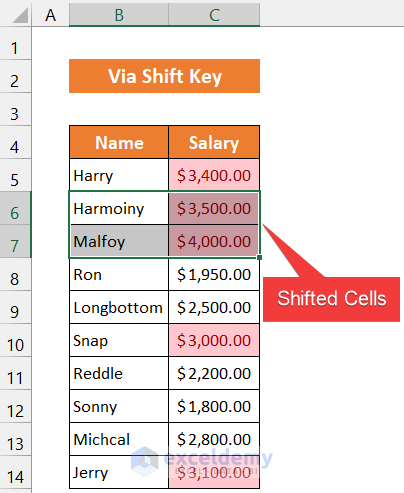
Follow the same procedure for the rest range of cells B10:C10 and B14:C14.
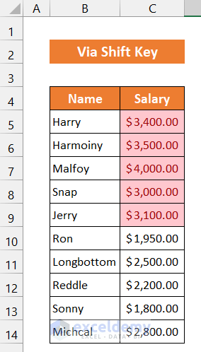
You will get all the highlighted cells at the top of your dataset.

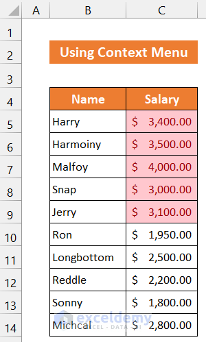
Method 5 – Utilizing the Context Menu

Steps:

Select the entire range of cells B4:C14.
In the Home tab, select Conditional Formatting.
Click on Highlight Cell Rules and choose Between.

A small dialog box called Between will appear.
Write down your desired lowest and highest salary amount like the image shown below. We chose the salary range of $3,000 to $4,000.
Choose the cell highlight pattern. We kept the default one, Light Red Fill with Dark Red Text.
Click OK to close the dialog box.

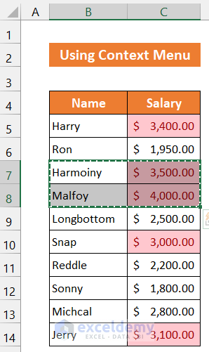
You will see the salaries within the range highlighted.
Select the range of cells B7:C8.
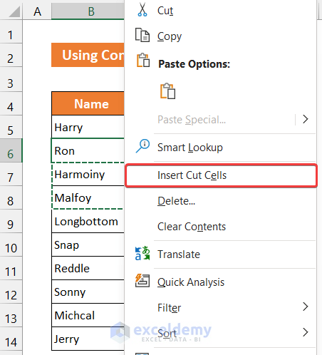
Press Ctrl + X on your keyboard.

Select cell B6.
Right-click and select the Inset Cut Cells option.

The range of cells will move upward.

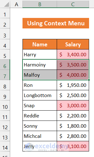
Do the same for the rest range of cells B10:C10 and B14:C14.
You will get all the highlighted cells at the top of your dataset.

Things You Should Know

If you have only a limited amount of highlighted cells to move, like our dataset, you can follow the manual approaches. Otherwise, we recommend you follow our first method. It will save you time.

Download the Practice Workbook

Move Highlighted Cells.xlsx