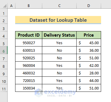
Suppose we have a dataset containing some Product ID, Delivery Status and Price of those products. We will show the way to find specific data from the dataset by creating a Lookup Table.
Method 1 – Applying the LOOKUP Function to Create a Lookup Table in Excel
Let’s find the Price of a Product ID from the dataset.
- Write the Product ID in cell F5.
- Select cell G5 where we want the Price to appear.
- Copy the following formula in that cell:
=LOOKUP(F5,B5:B11,D5:D11)- Press Enter. We will see the Price of the product with the Product ID in the lookup cell.
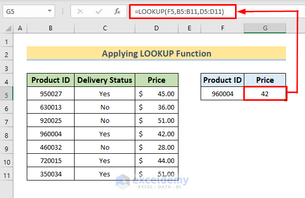
In the formula, we used the LOOKUP function with arguments,
- Cell F5 contains the value to look up.
- B5:B11 is the range where that value should be found.
- D5:D11 is the range where the corresponding result value is stored.
Read More: How to Create Table from Another Table in Excel
Method 2 – Inserting Excel VLOOKUP Function to Make Lookup Table
- Write the Product ID in Cell F5 whose Price we want to find.
- Select Cell G5 and copy the following formula in the cell:
=VLOOKUP(F5,B5:D11,3,FALSE)- Hit Enter.
In the formula, we used the VLOOKUP function with arguments,
- Cell F5 is the look-up value.
- B5:D11 is the range of data where the lookup value can be found.
- 3 is the column number from where the result will be picked.
- FALSE means the look-up value should be matched exactly.
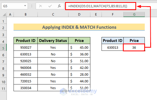
Method 3 – Combining INDEX & MATCH Functions for a Lookup Table in Excel
- Write the Product ID in Cell F5 whose Price you want to find.
- Input the following formula in Cell G5:
=INDEX(D5:D11,MATCH(F5,B5:B11,0))- Hit Enter.

In this formula,
- The MATCH function takes D5:D11 as an argument which is the range from where the function will find the desired value.
- And MATCH(F5,B5:B11,0) This part gives the row number as an argument of the MATCH function.
- In the MATCH function, F5 is the look-up value in the range B5:B11 and 0 means the match should be exact.
Method 4 – Generating Lookup Table with the HLOOKUP Function
Let’s find the fifth product’s Product ID:
- In Cell F5, write the name of the column from where we will pick the desired data.
- In Cell G5 write the formula given below.
=HLOOKUP(F5,B4:D11,5,0)- Press Enter.
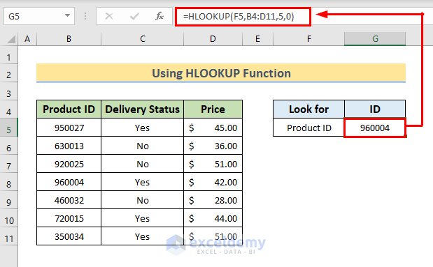
In the formula, we used the HLOOKUP function whose arguments are:
- Cell F5 contains the value to look for.
- B4:D11 is the table array where the function will look for the value.
- 5 denotes the desired value in the 5th row of the column where the lookup for value is found.
- 0 denotes the match should be exact.
Read More: How to Create Table from Another Table with Criteria in Excel
Method 5 – Using the XLOOKUP Function to Create a Lookup Table
- Write the Product ID in Cell F5 whose Price we want to find.
- Input the following formula in Cell G5:
=XLOOKUP(F5,B5:B11,D5:D11)- Press Enter.

In the formula of the XLOOKUP function we used the following cells as arguments,
- Cell F5 as the value to look for.
- B5:B11 is the range from where the function will find the value.
- D5:D11 is the range from where the function will find the matched output.
Download Practice Workbook
You can download the practice workbook from here to exercise.
Related Articles
- How to Mirror Table on Another Sheet in Excel
- How to Create Table from Multiple Sheets in Excel
- How to Make 3D Table in Excel
- How to Make a Decision Table in Excel
- How to Create a League Table in Excel
- How to Make a Table Bigger in Excel
<< Go Back to Excel Table | Learn Excel
Get FREE Advanced Excel Exercises with Solutions!
