Excel Practice & Exercises with INDEX-MATCH Formula

In this article, you will get eleven INDEX MATCH Excel practice exercises. Most of the problems are easy to solve. You will need an advanced level of Excel knowledge to solve all the problems. To solve all the problems, you should know about the following functions: INDEX, MATCH, CONCAT, CONCATENATE, and TEXTJOIN. Additionally, you will need to learn about the following things: examples with the INDEX-MATCH formula, use of the INDEX MATCH formula, INDEX-MATCH with multiple matches, INDEX MATCH for multiple results, the sort feature, and Excel VBA. You will need the latest version of Excel (Microsoft 365) to solve all the problems.

Download Practice Workbook

You can download the Excel file from the following link.

Problem Overview

There are eleven Excel INDEX MATCH related practice exercises in this file. The datasets are all different for each of the problems. You should open the Excel file and go through the problem statements. The exercises are provided in the “Problem” sheet, and the solutions to those are in the “Solution” sheet. Moreover, the first exercise is shown in the following picture.

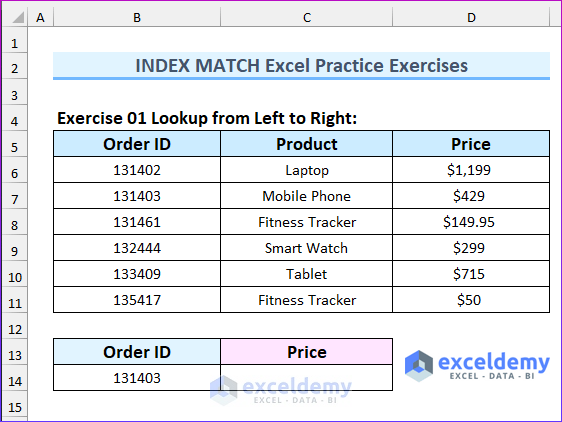
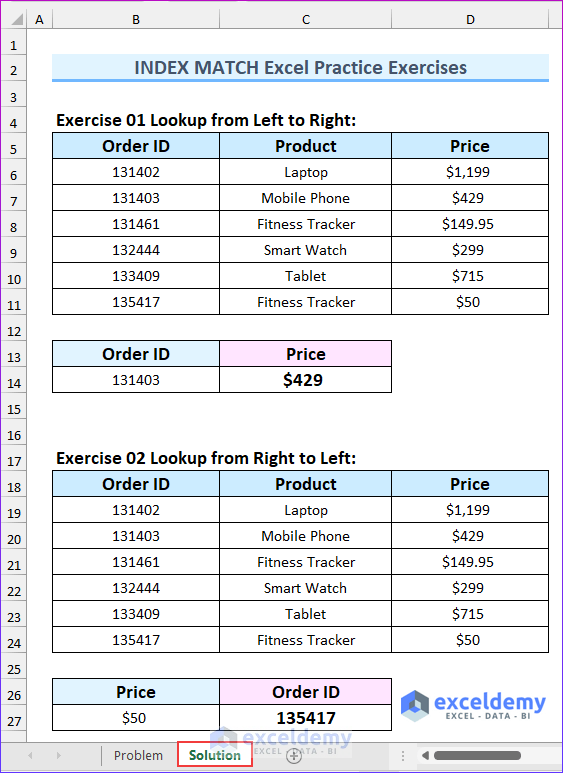
• Exercise 01 Lookup from Left to Right: Find the price of a specific Order ID (131403).

The animated image below shows the formula to solve the first problem.

• Exercise 02 Lookup from Right to Left: Lookup the Order ID from a specific price ($50). This time, you will search for data from the right side to the left side.
• Exercise 03 Lookup Two Columns (Array Formula): Use an array formula to search data from two columns (Product and Order ID) and return a single output (Price).
• Exercise 04 Two Way Lookup: Apply the MATCH function twice to find the product name from an order ID (133409) and column name (“Product”).
• Exercise 05 Lookup with Partial Match: In this exercise, find the price of a partially matched product name (“Lap”) using a wildcard character(*).
• Exercise 06 Multiple Criteria Lookup: Use a different formula than the exercise 03 to find the price of a product sold (“Mobile Phone”) by a specific salesman (“Aaron”). Hint: use a multiplication formula inside the lookup_array of the MATCH function.
• Exercise 07 Retrieve Values of Entire Row: Create a formula to return the row values of a salesman named “Dexter”.
• Exercise 08 Find Approximate Match: Find the product name from the nearest price given ($450). Remember, you need to sort your data to use this formula.
• Exercise 09 Multiple Criteria Without Array Formula: Find the student who got 100 in both the subjects. You need to use a helper column to do this.
• Exercise 10 Use of VBA INDEX MATCH: Apply VBA code to return the Gender and Country name for the student named “Samuelson”. You can press Alt+F11 to bring up the VBA window. Additionally, you can enable the Developer tab to do this.
• Exercise 11 Find Upcoming Event: Five people’s names and birthdays are given. Additionally, the current date is shown. Combine the functions to create two formulas to return the name and date of an upcoming birthday.

The following image shows the answers to the first two exercises.

Conclusion

Thank you for reading this article. By completing these practice exercises, we hope that you have gained knowledge about the INDEX MATCH functions of Excel. Moreover, you can find more articles similar to this on the ExcelDemy website. Additionally, if you have any questions or suggestions, feel free to comment below. However, remember that our website implements comment moderation. Therefore, your comment may not be instantly visible. So, have a little bit of patience, and we will solve your query as soon as possible. Keep excelling!