How to Create a Project Roadmap in Excel (4 Methods)

Method 1 – Using Shapes

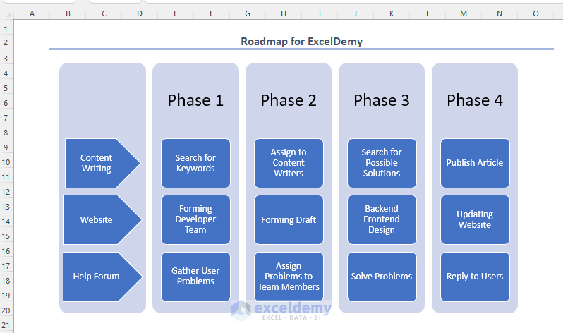
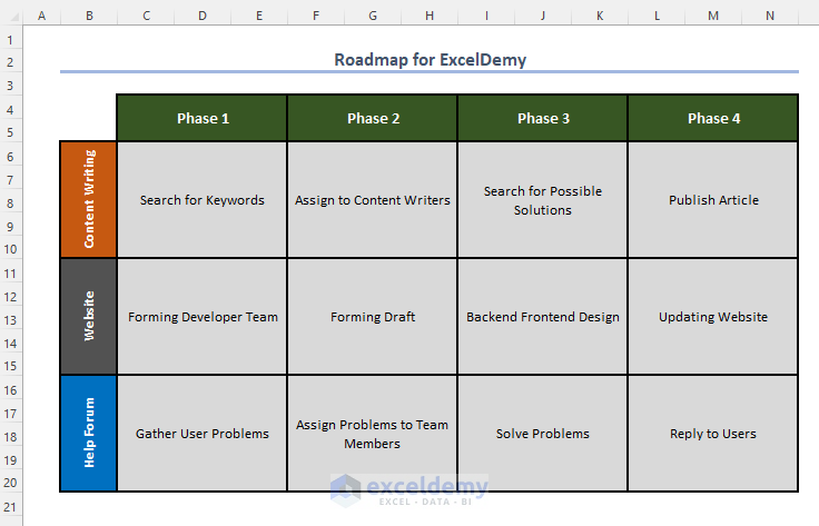
In the following sheet, we will create a Roadmap for ExcelDemy using different shapes in Excel.

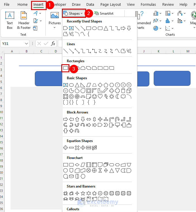
Step 1 – Insert Shapes

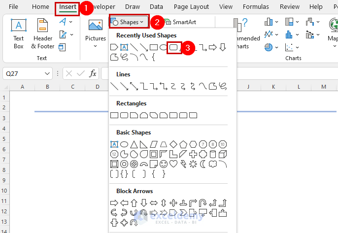
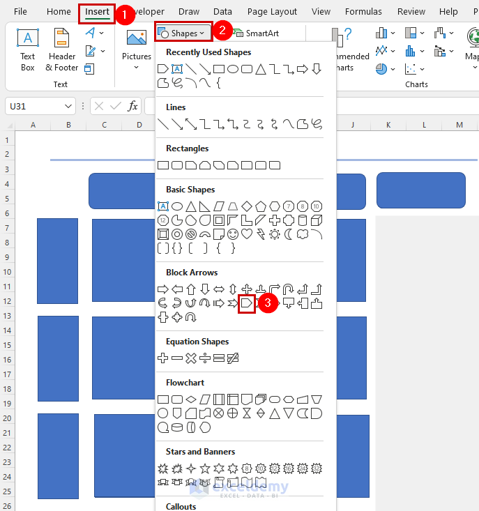
• Navigate to the Insert tab.
• Click on the Shapes dropdown menu.
• Choose Rectangle: Rounded Corners.

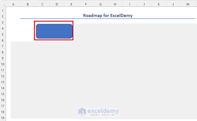
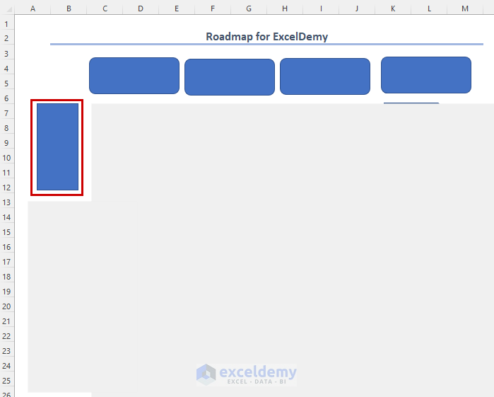
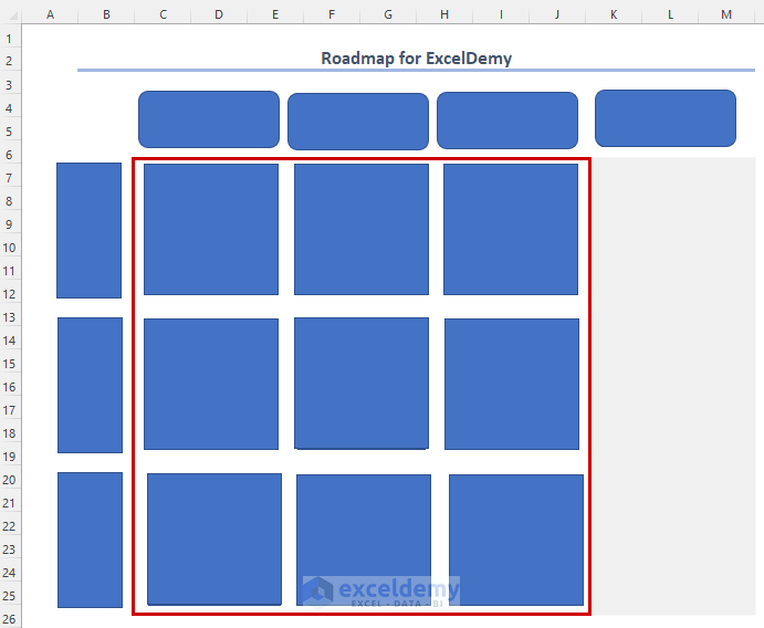
• Place the rounded rectangle shape where needed.

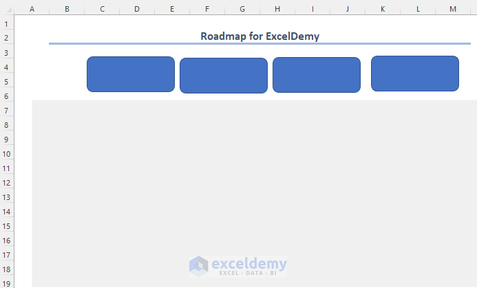
• Copy and paste this shape three times, arranging them sequentially in a line.

• Select a vertical rectangular shape from the Shapes dropdown.

• Place the rectangle vertically in the desired position.

• Insert two more rectangle shapes in the same line.

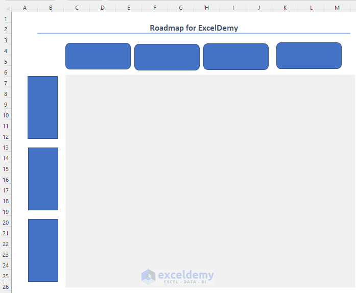
• Align the rectangular boxes between the shapes created in step 1.

• Ensure they are in line with the upper and side shapes.

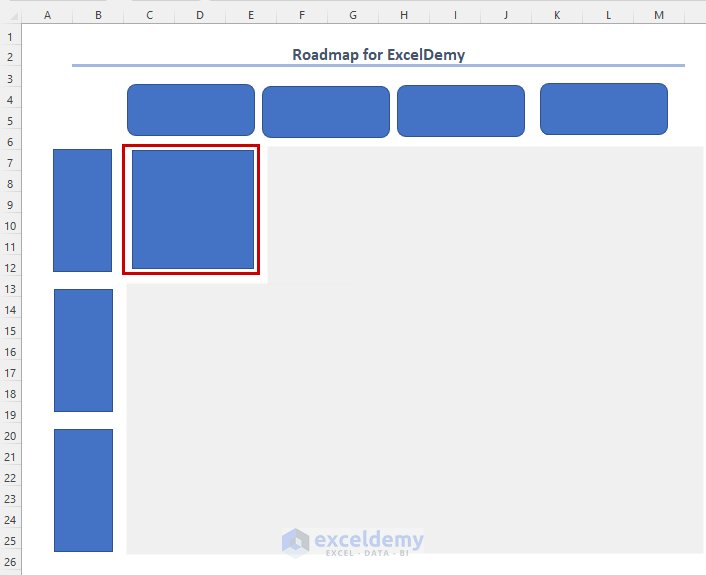
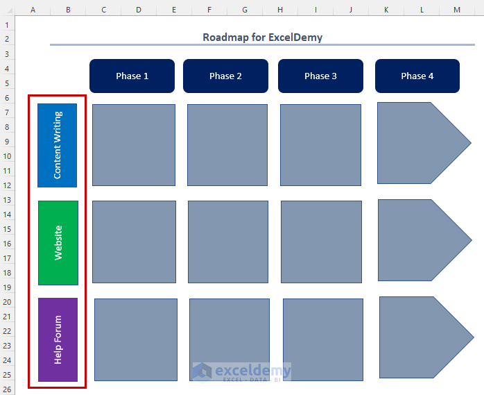
We completed the following shapes and aligned them with the upper and side shapes.

• To make the roadmap visually appealing, add a different shape to represent the final stage.
• Go to the Insert tab and choose Arrow: Pentagon.

• Position this arrow shape as indicated.

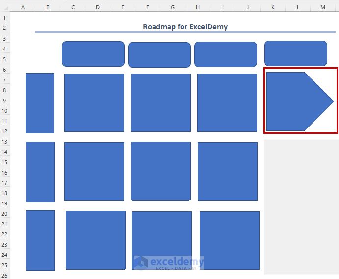
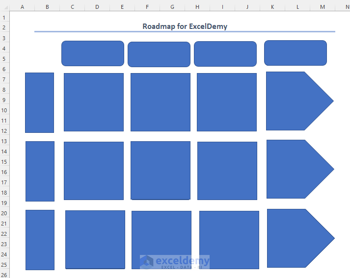
• Copy and paste the arrow shape into the last two empty spaces, aligning them in line.

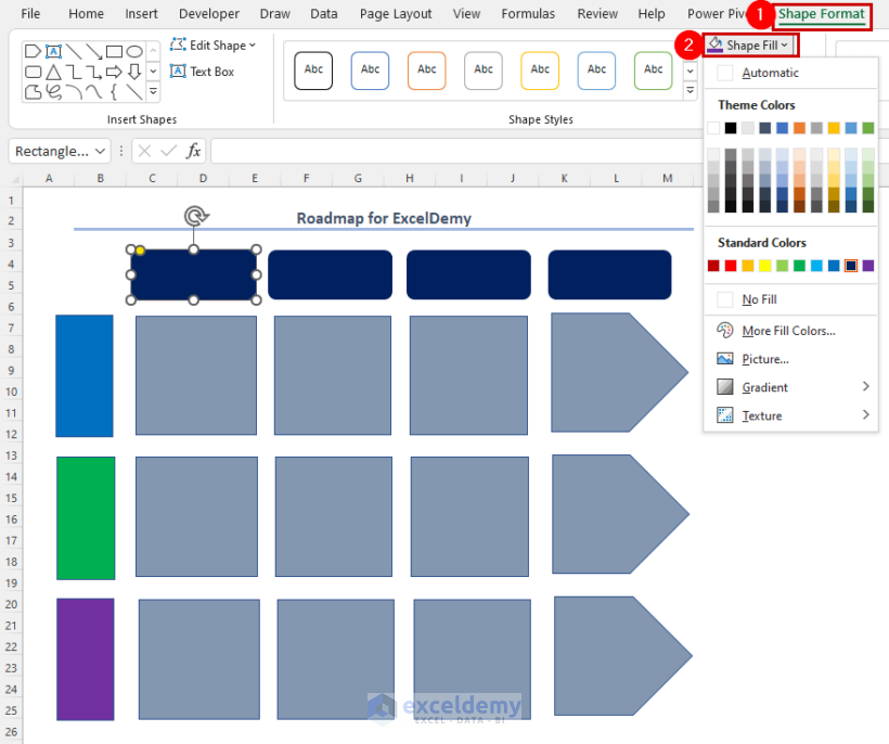
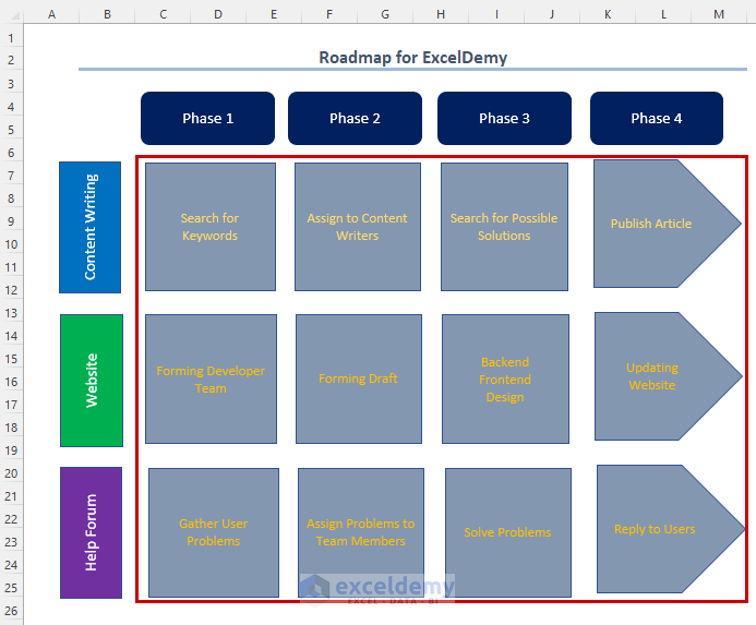
Step 2 – Customize Colors and Add Content

• Change the colors and formatting of the boxes.
• Select a shape, go to the Shape Format tab, and choose a color from the Shape Fill dropdown.

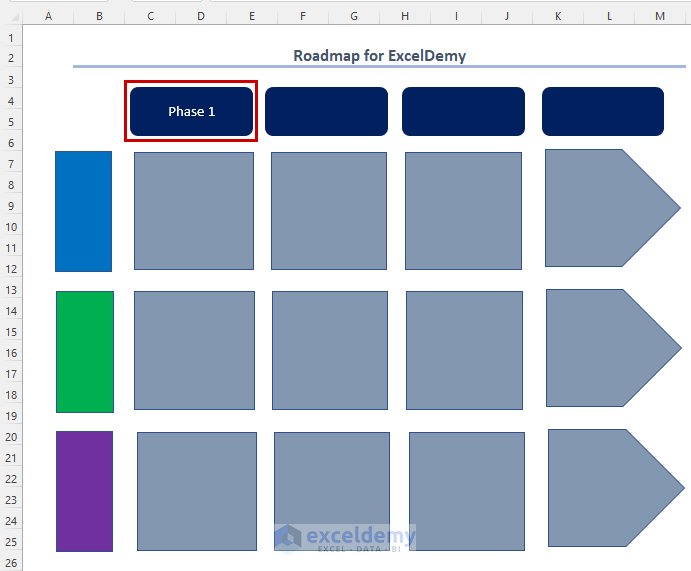
• Add content inside the shapes:
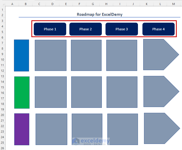
  • The first four shapes represent phases, so label them accordingly (e.g., Phase 1).

• Enter the other phase names for the rest of the cells.

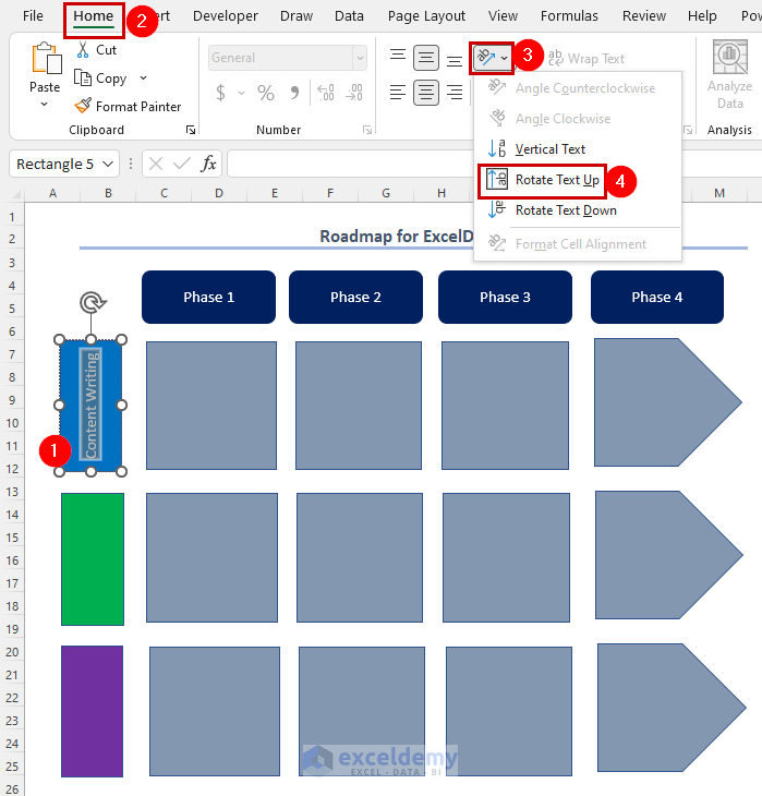
• Enter project names in the vertical boxes (e.g., Content Writing).
• Adjust text alignment as needed (e.g., use Rotate Text Up in the Home tab).

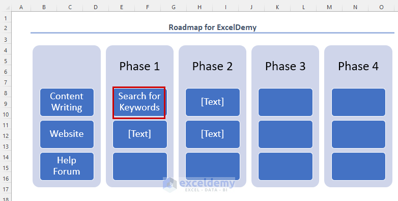
• Describe the work context for each phase and project (e.g., Search for Keywords).

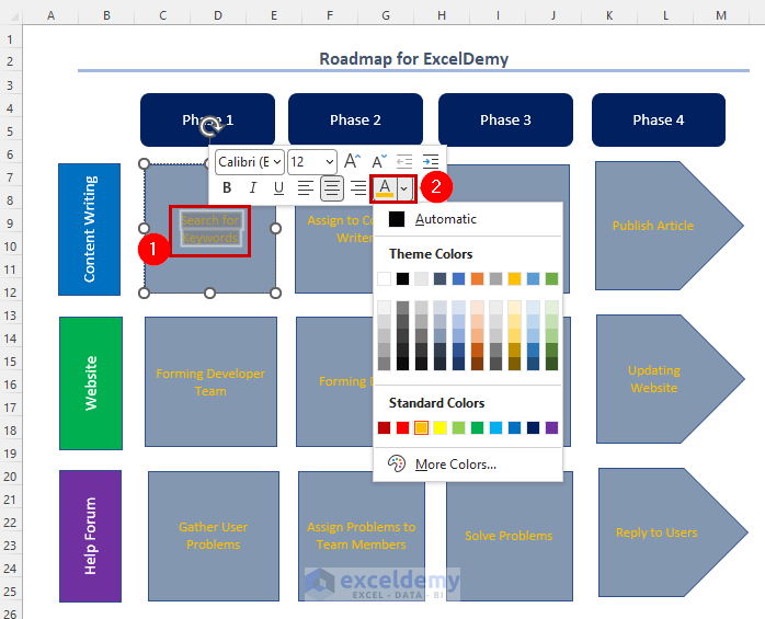
• If desired, modify the content color of the boxes:
  • Right-click on the text.
  • Select the Font Color dropdown and choose a color.

Read More: How to Make a Venn Diagram in Excel (3 Easy Ways)

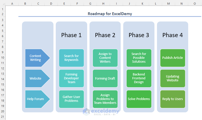
Method 2 – Applying SmartArt Graphics

Step 1 – Insert SmartArt Grouped List

• Navigate to the Insert tab.
• In the Illustrations group, click on SmartArt.

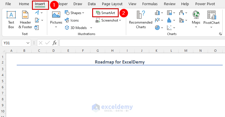
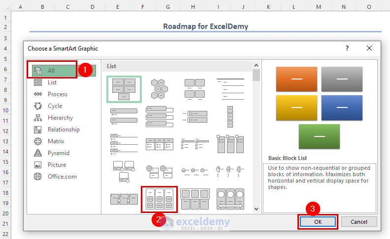
• The Choose a SmartArt Graphic window will appear.
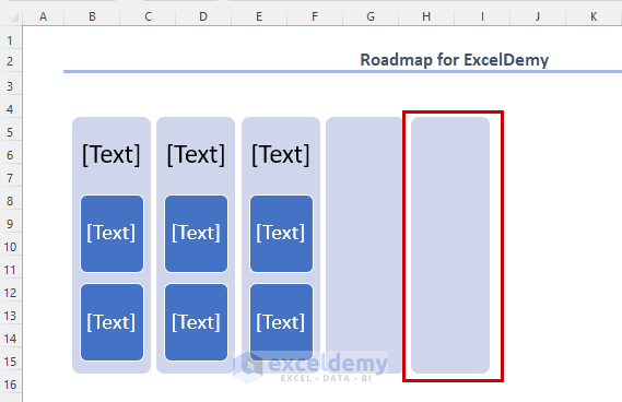
• Select the All tab and choose the Grouped List option.
• Press OK to insert the grouped list.

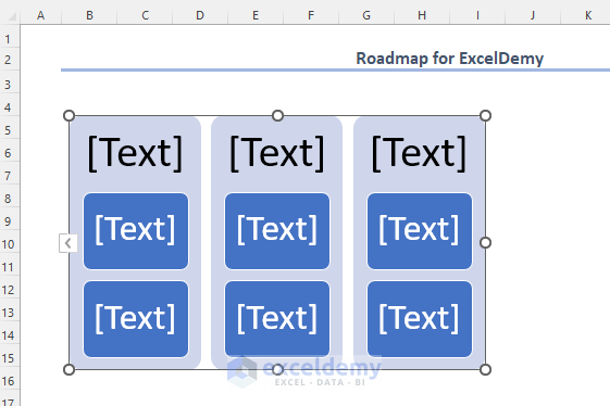
• As we need two more columns for our roadmap, follow these steps:
  • Select the list.
  • Go to the SmartArt Design tab and click Add Shape.

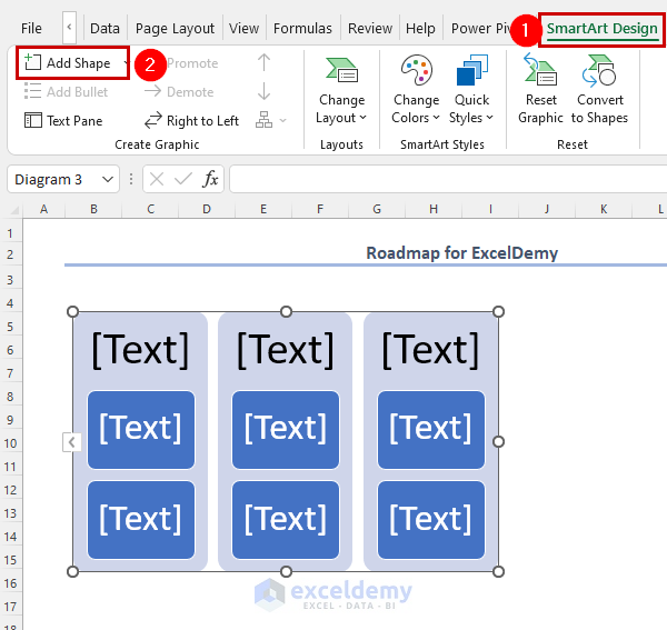
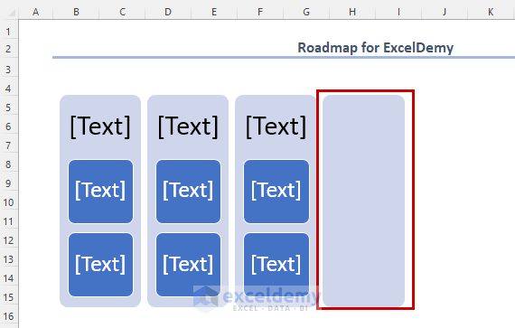
Repeat this process to insert another extra column.

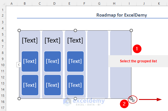
• Extend the size of the grouped list to accommodate the content inside the boxes:
  • Select the grouped list.
  • Drag the indicated symbol to the right and down.

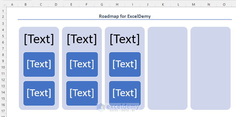
We extended the size of the grouped list.

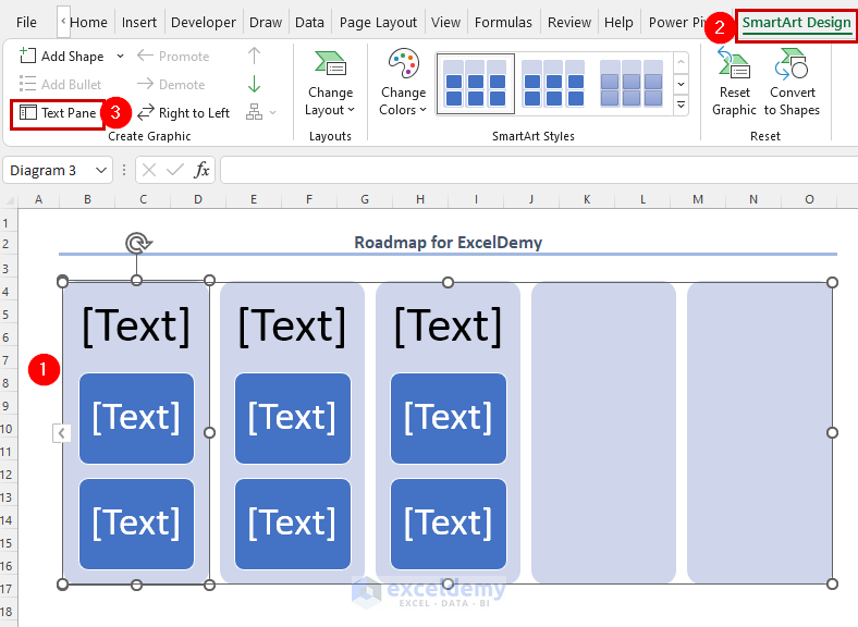
• To display the text pane:
  • Select the grouped list.
  • Go to the SmartArt Design tab and click on Text Pane.

Read More: How to Add SmartArt Graphics in Excel (7 Suitable Examples)

Step 2 – Insert Text Boxes

Add three text boxes in each column:

• Increase the number of text boxes from 2 to 3.
• Press ENTER after the 2nd line of the 1st column in the text pane.

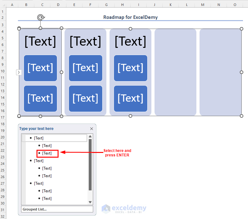
We entered an extra text box in the first column.

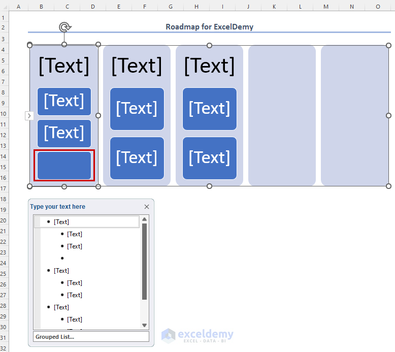
Add an extra text box in the next 2 columns.

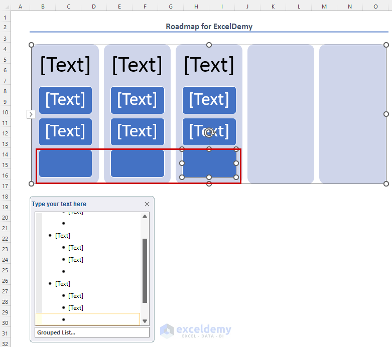
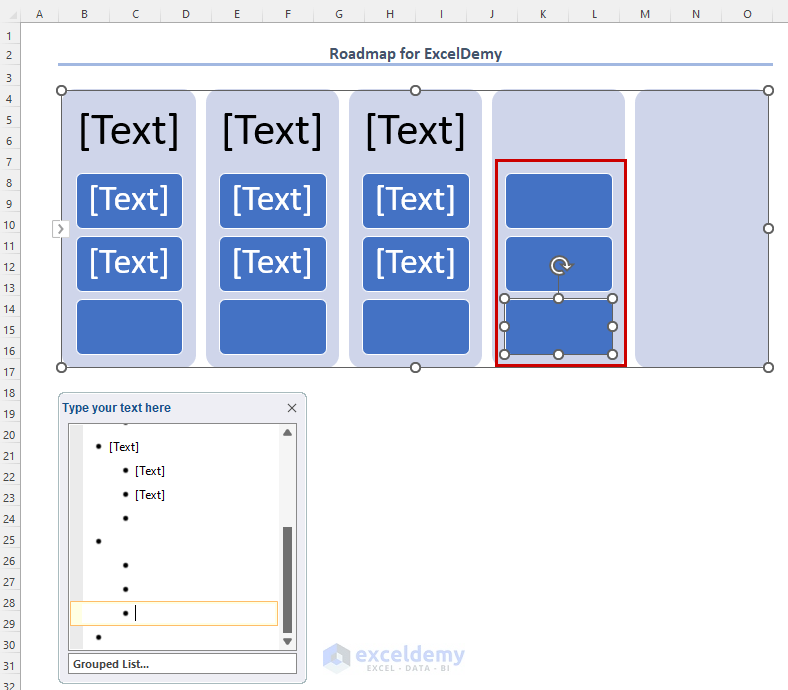
• We will enter 3 text boxes in the last newly added shapes.
• Click on the place of the 4th column in the text pane, and press ENTER.
• A new shape will be inserted.

• Press TAB.

• By pressing the TAB key, the newly added shape has been converted into a text box inside the previous shape.
• Press ENTER twice to add two new text boxes.

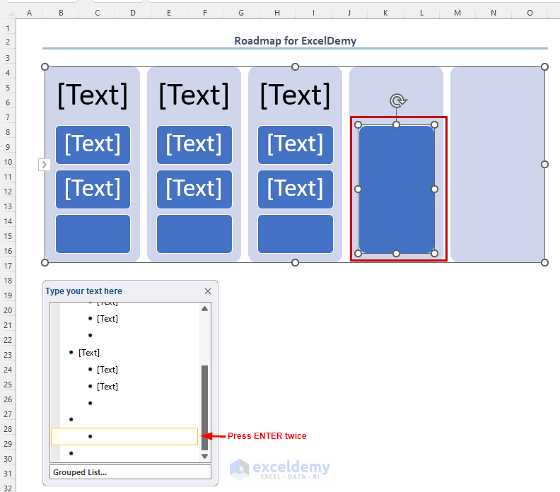
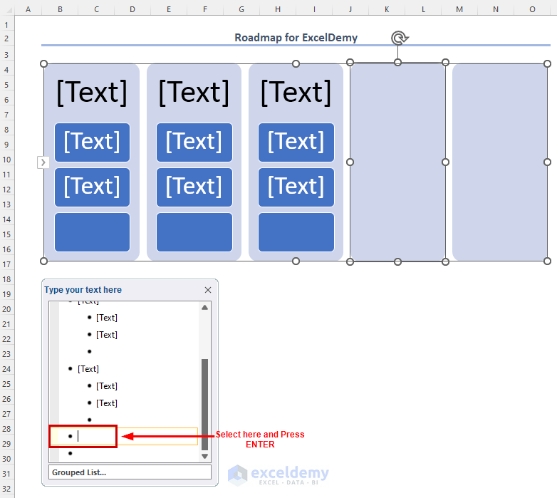
We successfully added the three text boxes in the 4th column.

• Follow the same process for column 5.

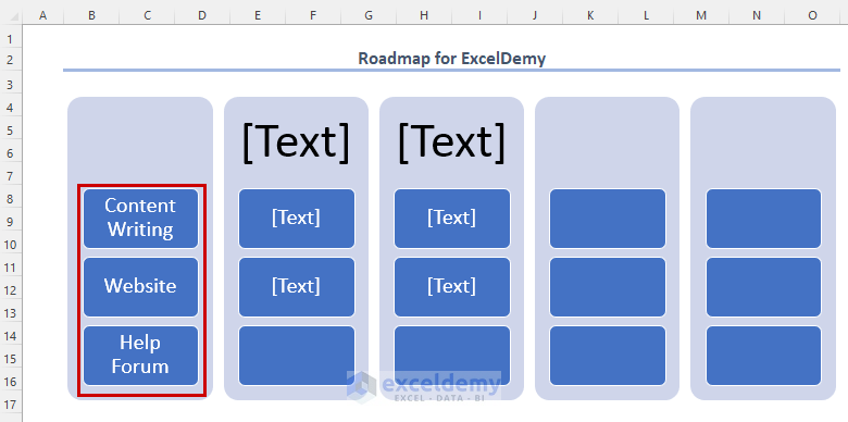
Step 3 – Enter Text Contents

• Enter project names in the first column.

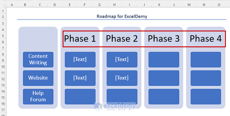
• In the headings of the next 4 columns, add phase numbers serially.

• To adjust font size as needed, select the text, right-click and change the font size.

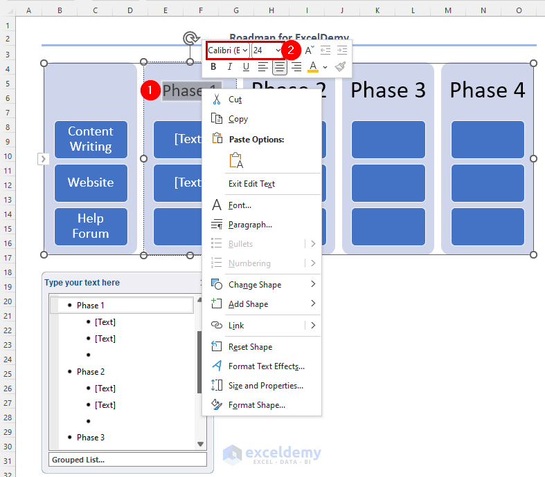
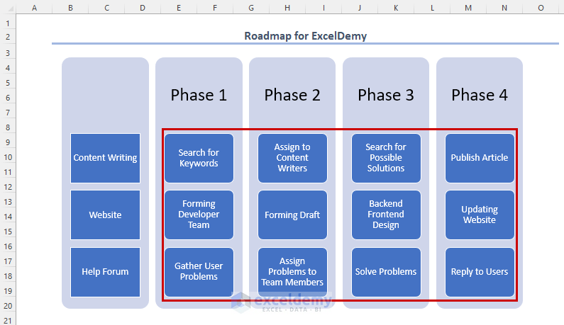
• Describe work contents for different phases and projects (e.g., Search for Keywords).

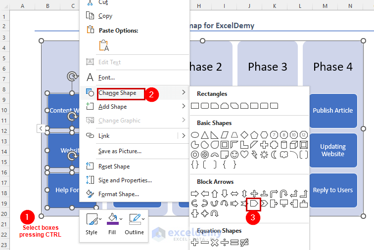
• Change the shapes of the project name boxes:
  • Select the boxes, right-click, and choose Change Shape (e.g., arrow symbol).T

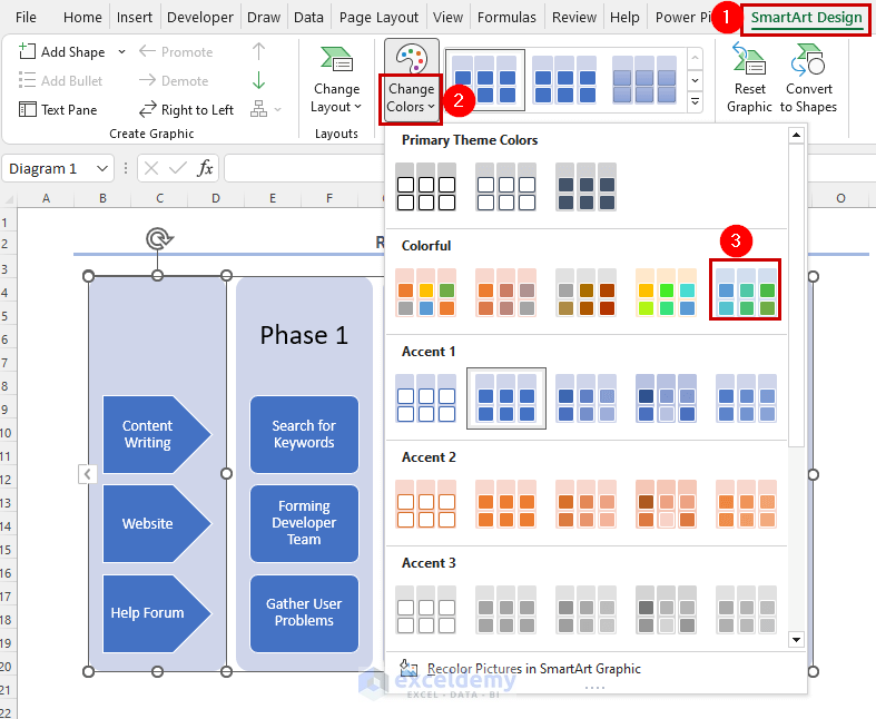
Optionally, modify the colors of the grouped list:

• Select the grouped list.

• Go to the SmartArt Design tab and choose a style from the Change Colors dropdown.

You’ve created the following Roadmap for ExcelDemy.

Read More: How to Insert WordArt in Excel (2 Simple Methods)

Method 3 – Modifying Cell Borders

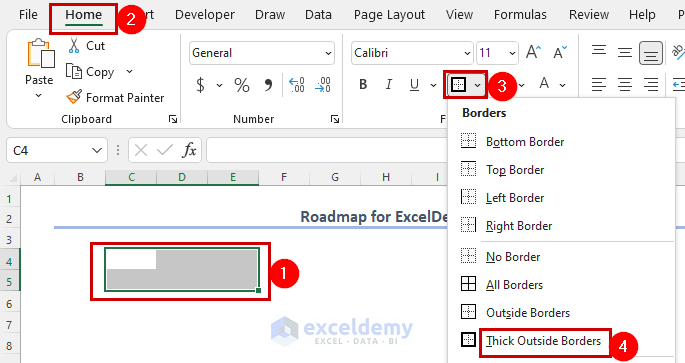
• Create Boxes for Phases:
  • Select 2 rows and 3 columns to create a box.
  • Go to the Home tab and click on the Borders dropdown.
  • Choose Thick Outside Borders to create the first phase box.

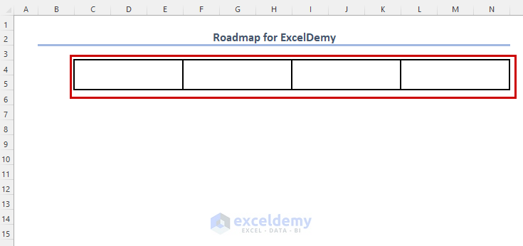
• • Repeat this process for the remaining phase numbers.

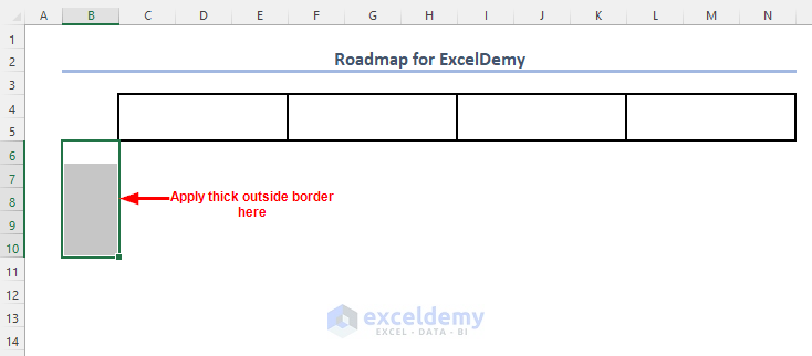
• • Vertically select 5 rows and apply thick outside borders for the project name boxes.

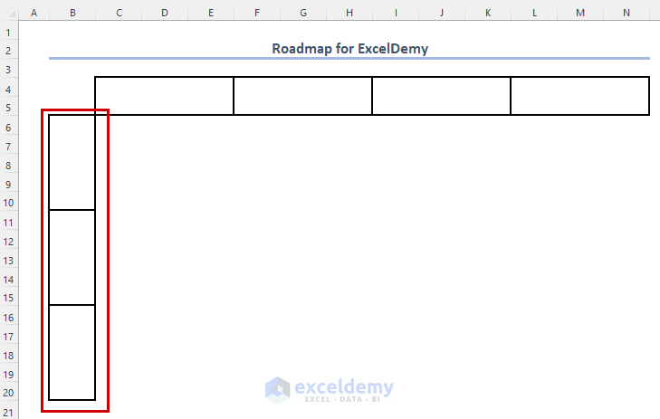
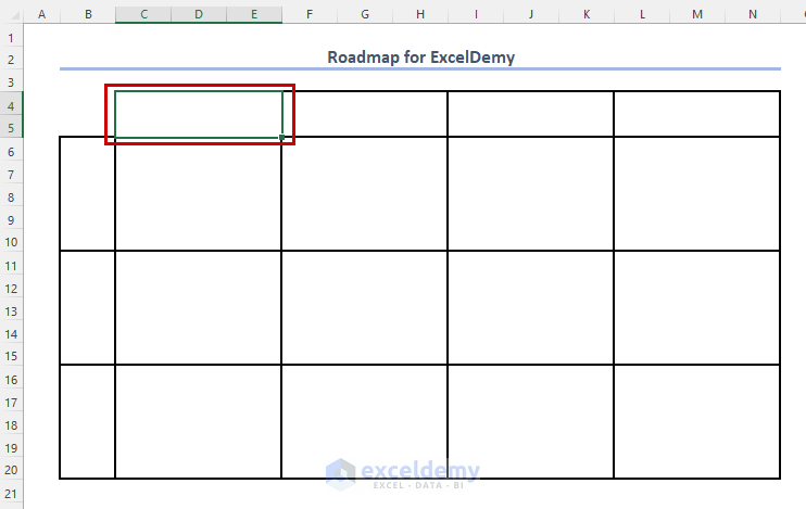
• Outline and Merge Cells:
  • Complete the outline of the boxes for project names.

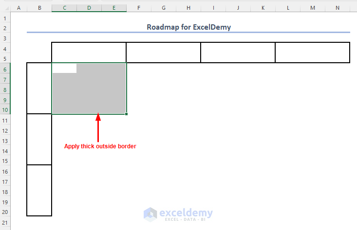
• • To enter work contents, select cells up to the intersection point of the first horizontal box and vertical box.
  • Apply thick outside borders to these cells.

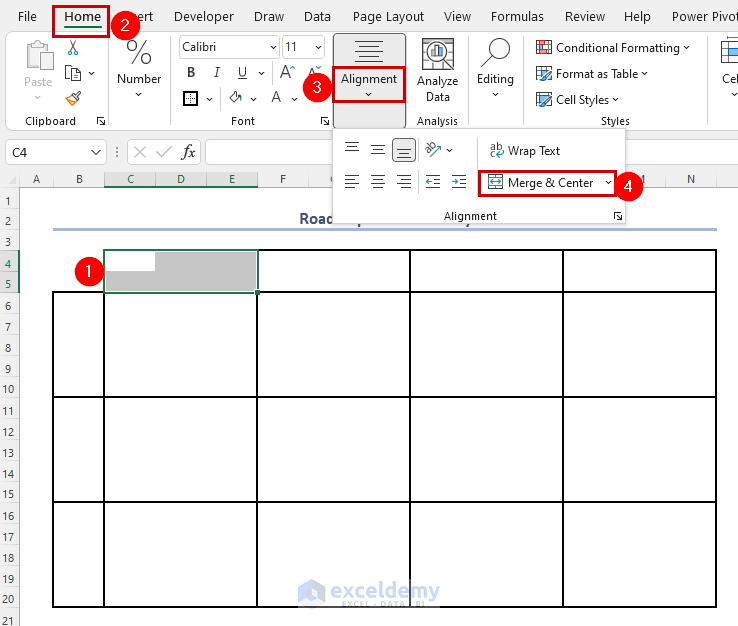
• Merge the cells within each box:
  • Select all cells of a box.
  • Go to the Home tab and click on Alignment dropdown.
  • Choose Merge & Center.

• Add Contents and Adjust Font Sizes:
  • Enter contents in the boxes.
  • Adjust font sizes as needed.

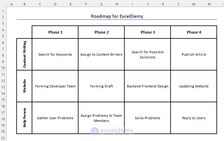
• Customize Colors:
  • Change the colors of the boxes to achieve the desired look.

Read More: How to Color Code Cells in Excel (3 Efficient Methods)

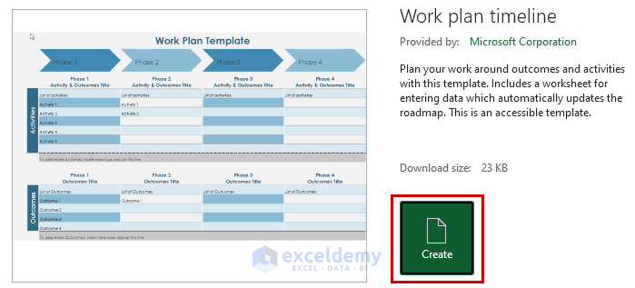
Method 4 – Using an Excel Template

• Ready-Made Templates:
  • Go to the File tab.

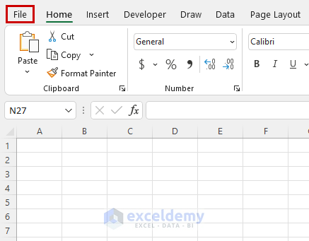
• • Enter Roadmap in the search bar.

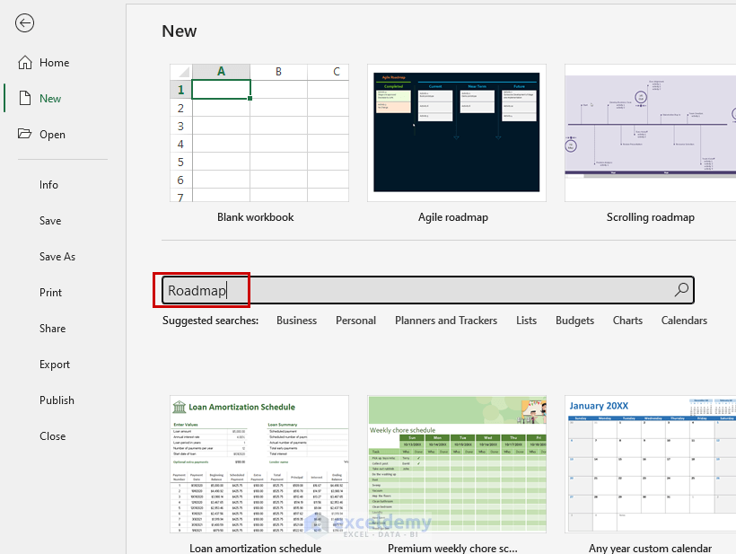
• • Different roadmap templates will appear.
  • Select your preferred template (e.g., Work plan timeline).

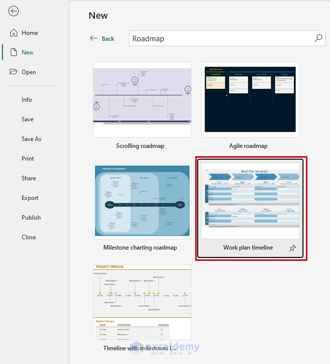
• • Click Create.

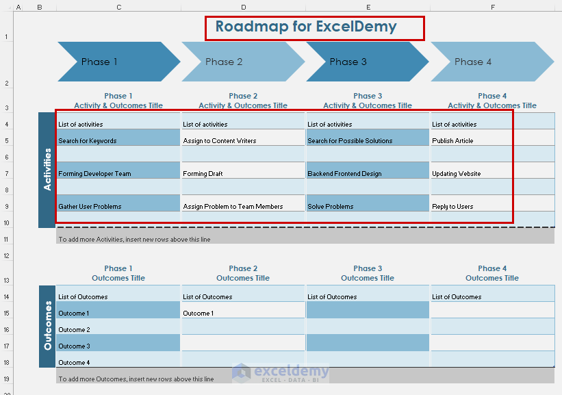
• Customize the Template:
  • You’ll be taken to a newly created workbook.
  • Go to the Work Plan sheet.

• • Change the title of the roadmap.
  • Enter activity names for the 4 different phases.
  • Add work outputs in the second box.

Download Practice Workbook

You can download the practice workbook from here:

Related Articles