How to Make a Recalculate Button in Excel (5 Easy Steps)

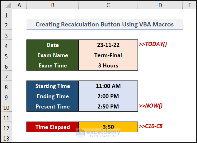
The Recalculate button allows you to update formulas in your dataset. If you’re using volatile functions that change over time, you’ll need to recalculate the formulas. Fortunately, you can achieve this with a simple button using VBA macros. Let’s dive into the easy steps for creating a Recalculate button in Excel:

Step 1 – Create a VBA Module

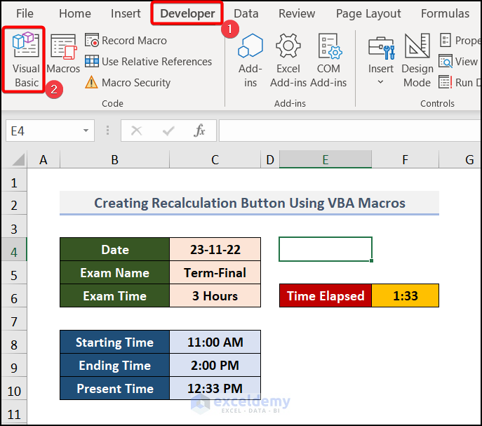
• Go to the Developer tab and select Visual Basic.

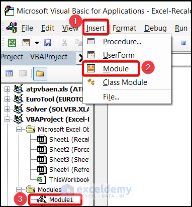
• Click on the Insert tab, choose Module, and create a new module (e.g., Module1).

• Enter the following VBA code in the module:

Sub RecalculateActivesheet()
  ActiveSheet.Calculate
End Sub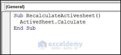

Read More: How to Recalculate in Excel

Step 2 – Insert the Recalculate Button

• Hover over the Developer tab and navigate to the Insert command in the Controls section.
• Choose a Button from the Form Controls options.

• An Assign Macro dialog will appear; click OK.

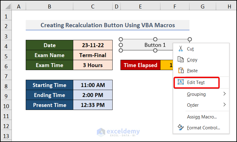
• A new button (Button 1) will be created. Right-click on it and select Edit Text to rename it (e.g., Recalculate).

Step 3 – Modify the Button’s Appearance

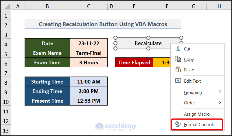
• Right-click on the button and choose Format Control from the Context Menu.

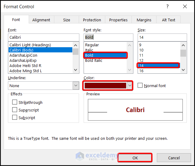
• In the Format Control window, select Bold for the font style, set the Size to 14, and choose your preferred Color. Click OK.

Step 4 – Assign the Macro to the Recalculate Button

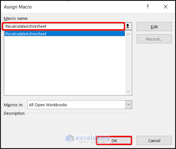
• Right-click on the button again and select Assign Macro.

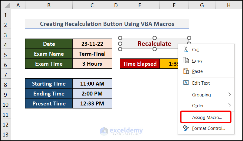
• In the Assign Macro window, enter the macro name as RecalculateActivesheet and click OK.

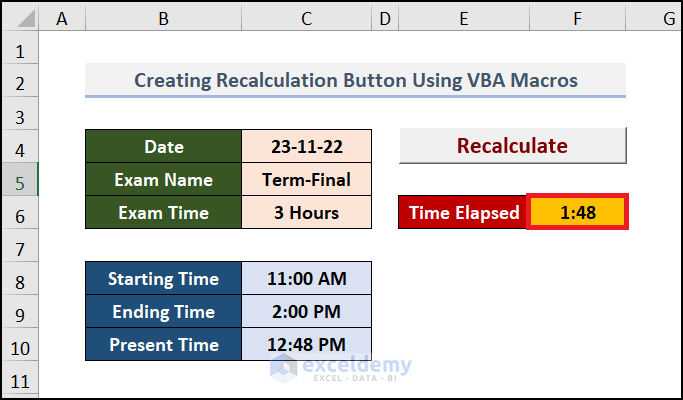
Step 5 – Test the Recalculate Button

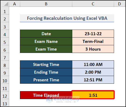
• Click the Recalculate button (as shown in the image).

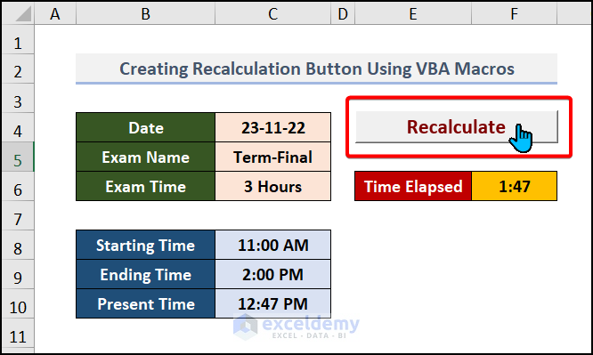
• The Time Elapsed will be recalculated each time you click the button.

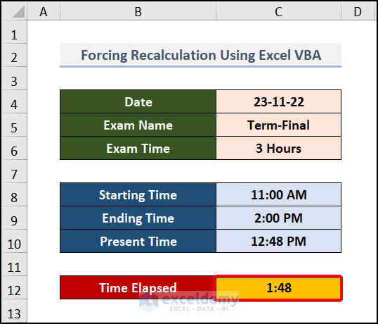
Forcing Recalculation Using Excel VBA

You can also forcefully recalculate the worksheet formulas using VBA code. Follow these steps:

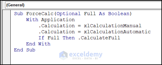
• Run the following code (press F5 in the module):

Sub ForceCalc(Optional Full As Boolean)
    With Application
        .Calculation = xlCalculationManual
        .Calculation = xlCalculationAutomatic
        If Full Then.CalculateFull
    End With
End Sub

This code was found on Folkstalk.com.

• Select the sheet name in the Macros window and click Run.

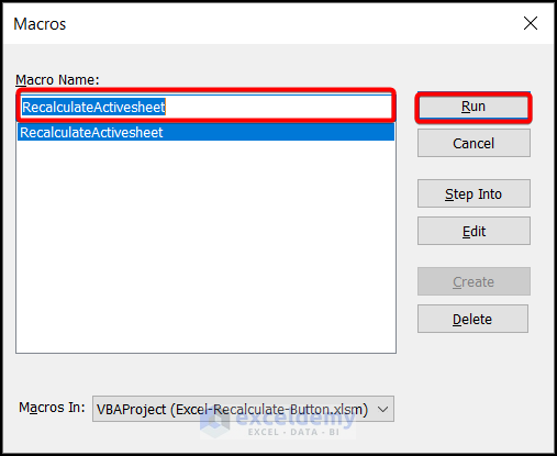
• The Time Elapsed will be updated (as shown in the image).

Read More: How to Force Recalculation with VBA in Excel

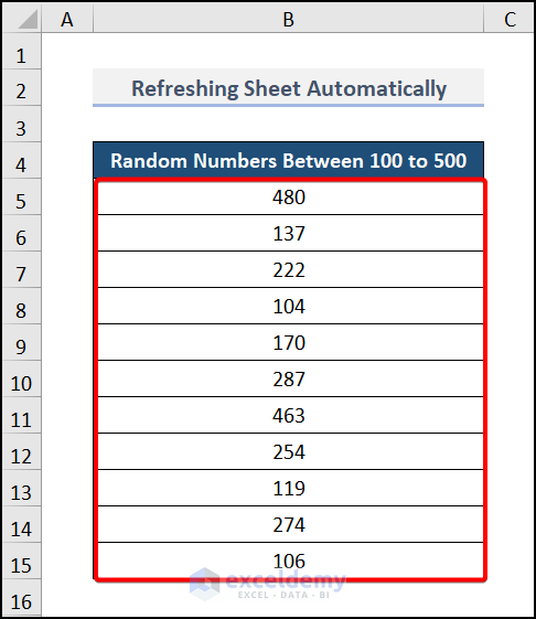
How to Refresh an Excel Sheet Automatically

To automatically refresh dataset numbers, use the keyboard shortcut:

• Take a dataset of random numbers generated by the RANDBETWEEN function (e.g., in cells B5:B15).

.

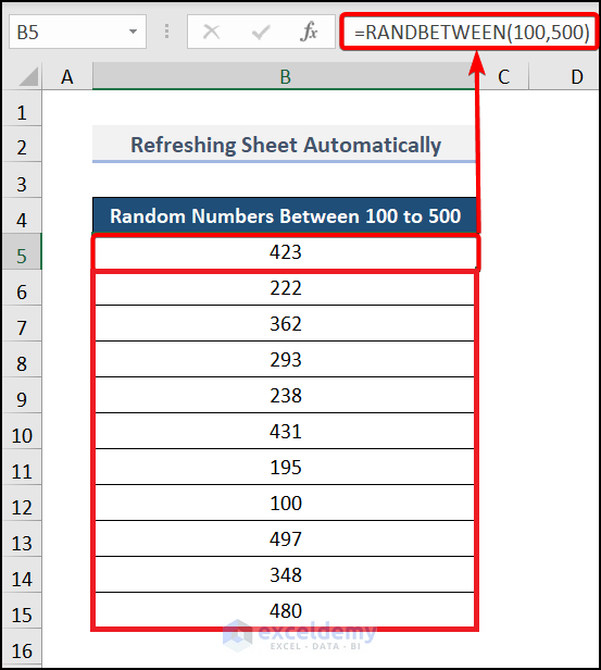
• Press the F9 key to refresh the random numbers automatically.

Download Practice Workbook

You can download the practice workbook from here:

<<Go Back to Excel Calculation Options | How to Calculate in Excel | Learn Excel