How to Highlight with Cursor in Excel (3 Suitable Ways)

If you are looking to highlight the cursor position before entering data into the cell or working with a lot of data and are at risk of losing track of where your cursor is, then you are in the right place. In this tutorial, you will learn 3 useful ways to highlight rows, columns, or both with the cursor in Excel.

How to Highlight with Cursor in Excel: 3 Suitable Ways

Our main goal is to highlight a row or column or both row and column simultaneously with the cursor. We will use the following dataset to describe the whole article.

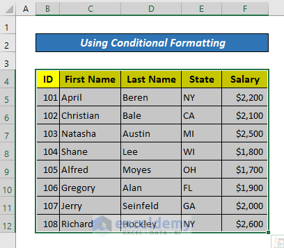
1. Use Conditional Formatting to Highlight Active Row and Column

If you want to highlight the selected row or/and column without using any VBA code, the best you can do is use conditional formatting. After applying the formula in conditional formatting, the first cell of our selected dataset is highlighted. Then, if you select another cell and press F9, the sheet is refreshed, the formula is recomputed, and the highlighting is updated.

This method is not as smooth as the VBA method (discussing next) as it requires recomputing the sheet manually. However, if you don’t want to use a macro-enabled Excel file, use one of the following ways as per your needs.

1.1 Highlight Active Row

To highlight the active row, just follow the steps below.

📌 Steps:

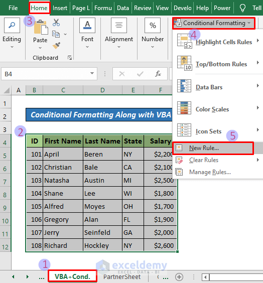
• First, select the entire dataset which you want to highlight. Then go to the Home tab >> Conditional Formatting button under the Styles group >> click on the New Rule.

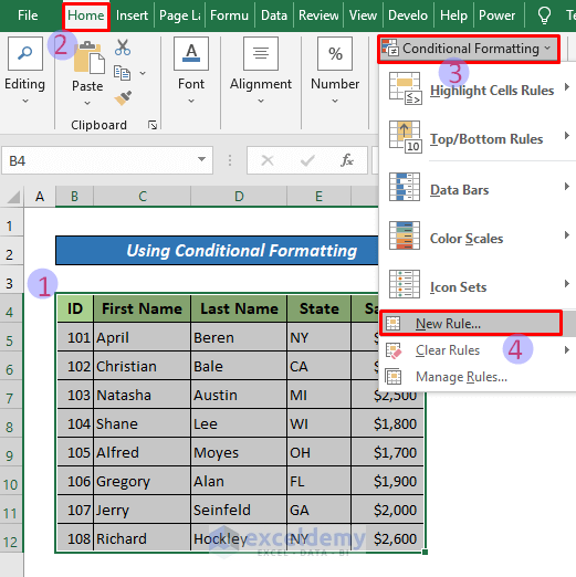
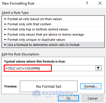
• A New Formatting Rule dialog box will appear.
• Click on the ‘Use a formula to determine which cells to format’ box. Type the following formula in the ‘Format values where this formula is true’ box. After that, click on the Format button.

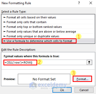
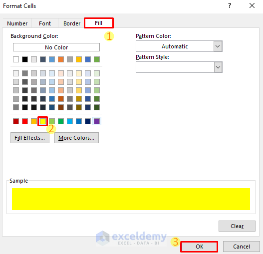
• In the Format Cells dialog box, under the Fill section, choose a highlighting color. Finally, press OK.

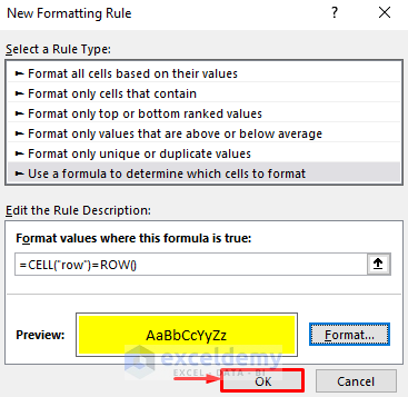
• It will return to the New Formatting Rule window again. At this time, just click on the OK.

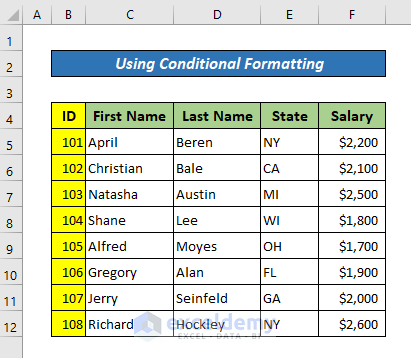
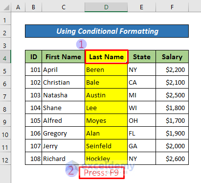
• Now, you will see that the 1st row of our dataset is highlighted.

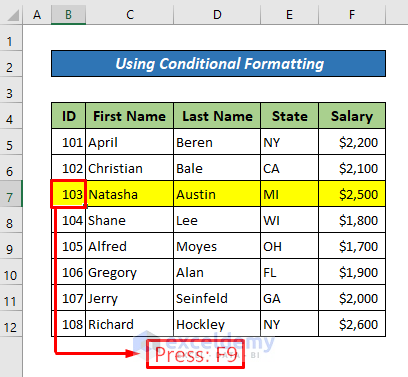
• If you want to highlight another row, just click on any cell of this row and press F9. Here is the result.

1.2 Highlight Active Column

To highlight an active column, repeat the steps above except the formula putting step.

• Copy the following formula and paste it into the ‘Format values where this formula is true’ box.

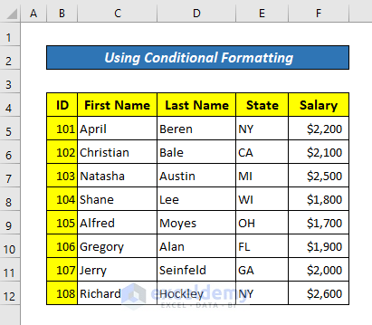
• After that, choose a highlighting color by clicking on the Format option.

• Here is the result. The first column of our dataset is highlighted.

• Now, if you want to highlight a new column, just click on any cell of this column and then, press F9. Look at the following image for the result.

1.3 Highlight Both Active Row and Column

• To get both column and row highlighted, you need to write the following formula in the formula box.

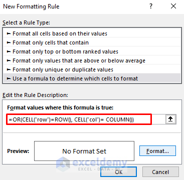
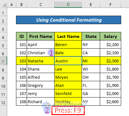
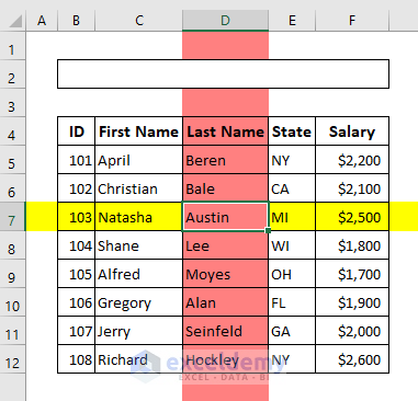
• Repeat all the steps as we stated before. You will get results like the following.

• Don’t forget to press the F9 key to apply highlighting after selecting another cell. 👇

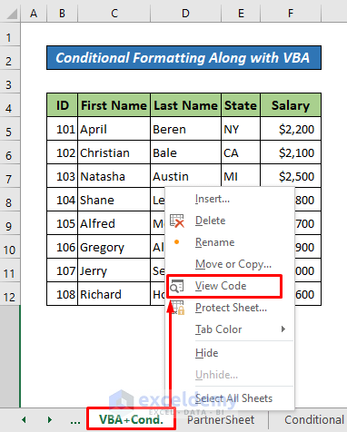
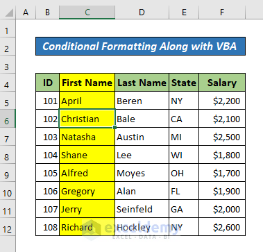
2. Apply Conditional Formatting Along with a VBA Code

To get rid of slowing down your workbook and recalculating a worksheet on every move, you can use VBA code to get the active row and column number, then put this number to the ROW and COLUMN function used in the conditional formatting formulas.

Follow the steps below to get the active row and column number using VBA codes. Before going, just open a new worksheet in your current workbook. And name that current worksheet as PartnerSheet.

📌 Steps:

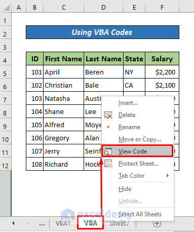
• First, right-click on the sheet name >> click on the View Code. A module window will pop up.

• In the module window, write down the following formula.

Private Sub Worksheet_SelectionChange(ByVal Target As Range)
Application.ScreenUpdating = False
Worksheets("PartnerSheet").Cells(3, 2) = Target.Row
Worksheets("PartnerSheet").Cells(3, 3) = Target.Column
Application.ScreenUpdating = True
End Sub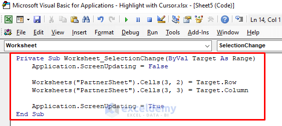

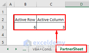
• Now, click on any cell in your dataset.

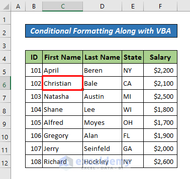
You can also see the row and column number of that cell in the PartnerSheet.

2.1 Highlight Active Row

After minimizing the VBA window, go back to the dataset, and select the whole dataset. Now, follow the steps below.

📌 Steps:

• Go to Home tab >> Conditional formatting >> New Rule.

• Click on the ‘Use a formula to determine which cells to format’ box. Type the following formula in the ‘Format values where this formula is true’ box. After that, click on Format to choose a formatting color.

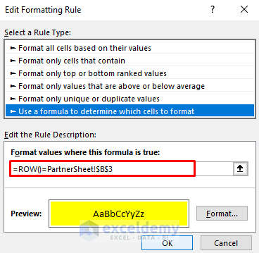
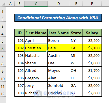
Finally, here is the result.

2.2 Highlight Active Column

To highlight a column, type the following formula in the formula box.

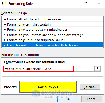
Now click on any cell to see the entire highlighted column of this cell.

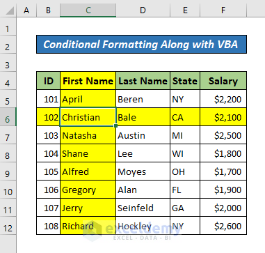
2.3 Highlight Active Row and Column Both

If you want to highlight both row and column simultaneously, copy the following formula and paste it into the formula box as shown in the following image.

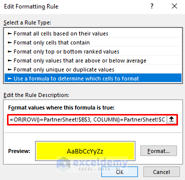
Finally, here is the result. Just click on any cell that you want to highlight both the row and column of that cell.

3. Use VBA Codes to Highlight with Cursor

If you are comfortable with VBA codes in Excel, then, there are available very efficient VBA codes that can help you to highlight both rows and columns in one click. We have discussed two VBA codes here for you to highlight with the cursor in Excel.

3.1 Highlight Multiple Rows and Columns with Union Function

In the first code, we will apply the Union function in VBA. This code will allow you to select and highlight multiple cells and their corresponding rows and columns.

To apply this magic trick, just follow the steps.

📌 Steps:

• First, right-click on the sheet name (where your dataset can be found), and select View Code. A module window will pop up.

• Now, copy the following codes and paste them into the VBA window of the specific worksheet. After that, minimize the window.

Private Sub Worksheet_SelectionChange(ByVal Target As Range)
Cells.Interior.ColorIndex = 0
Union(Target.EntireColumn, Target.EntireRow).Interior.ColorIndex = 34
End Sub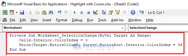

• Click on any cell of your dataset. You will see the entire row and column of that cell highlighted.

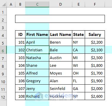
If you want to highlight multiple rows and columns by selecting multiple cells, you can do this by using the same VBA code. If your cells are not next to each other, then use CTRL to select multiple cells.

3.2 Highlight Single Row and Column

This code will highlight only one row and one column at a time.

📌 Steps:

• Please, copy the following code and paste it into the VBA module (select your sheet from the Microsoft Excel Objects menu).

Private Sub Worksheet_SelectionChange(ByVal Target As Range)
If Target.Cells.Count > 1 Then Exit Sub
Application.ScreenUpdating = False
Cells.Interior.ColorIndex = 0
With Target
.EntireRow.Interior.ColorIndex = 27
.EntireColumn.Interior.ColorIndex = 22
End With
Application.ScreenUpdating = True
End Sub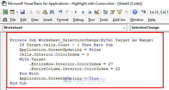

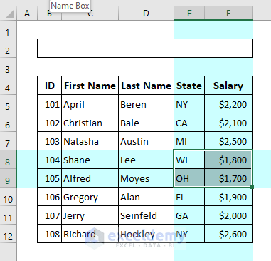
Finally, here is the result.

You can customize this code for color, in the following ways.

• The code uses 2 different colors, color index 27 for the row and 22 for the column. If you want to customize the color, just change the ColorIndex codes. 
• If you want to highlight the row and column with the same color, use the same color index.
• If you want to only highlight an active row, just delete the line below,

.EntireColumn.Interior.ColorIndex = 22

• If you want to only highlight an active column, just delete the line below,

.EntireRow.Interior.ColorIndex = 27

Read More: How to Move Cursor in Excel Cell

Download Practice Workbook

You can download the following practice workbook that we have used to prepare this article.

Conclusion

In this tutorial, I have discussed 3 useful ways to highlight rows, columns, or both with the cursor in Excel. I hope you found this article helpful. Please, drop comments, suggestions, or queries if you have any in the comment section below.

Related Articles

• How to Move Cursor in Excel Cell
• Excel Cursor Movement: Logical vs Visual
• How to Change Cursor Color in Excel
• [Fixed!] Excel Cursor Locked in Select Mode
• [Fixed!] Excel Cursor Stuck in Drag Mode
• [Fixed!] Excel Cursor Stuck on White Cross

<< Go Back to Cursor in Excel | Excel Parts | Learn Excel