How to Use TRUE Function in Excel (10 Ideal Examples)

The TRUE function has a special type of compatibility in returning results based on logical conditions.

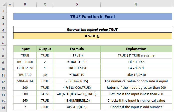
TRUE Function in Excel (Quick View)

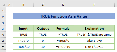
Example 1 – Apply TRUE Function as Value

The TRUE function acts as a logical value in Excel. So that you can use the function in calculations. The numerical value of TRUE is 1 during calculations as shown in the following image.

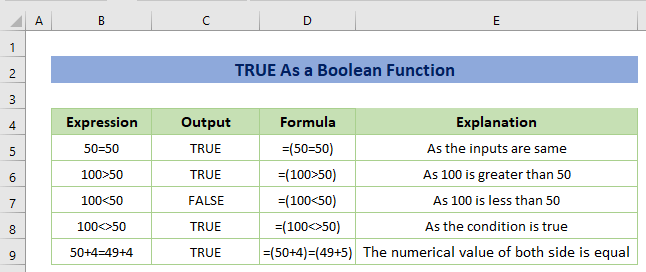
Example 2 – Use TRUE as Boolean Function

A Boolean variable can have one of two possible values. One possible value for a binary variable is 0 (false), while the other is 1.

The TRUE function returns the value 1 while acting as a Boolean function.

There are various types of expressions in the following figure. As the input is entered with the logical operator, the result displays TRUE if the logic is true. Otherwise, it shows FALSE.

A bit more complex example like the following will be used for illustration.

For example, the product names with their prices are given. Also, a criterion is provided that you have to find the discount for all products based on a discount of 15% for the price greater than $250.

If the logical statement says the price is greater than $250, the result will be TRUE, and also the TRUE will be replaced by the given percentage of 15%. For this, we’ll use the IF function.

The formula would be:

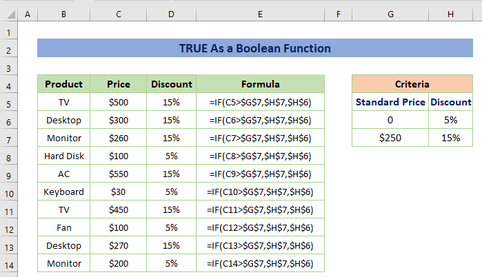
Example 3 – Finding Greater or Less Than Value from a Given Value

Suppose, the standard price is given as $200. Now you have to check whether the value is greater than $200 or not.

In this case, the formula would be:

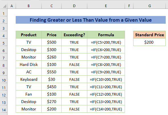
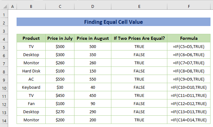
Example 4 – Finding Equal Cell Value

Let’s imagine you have two prices e.g. prices in July and prices in August and you have to check if the two prices are equal or not.

Enter the following formula in F5:

C5 is the price in July and D5 is the price in August.

Example 5 – Combine NOT Function with TRUE Function

Like the TRUE function, the NOT function is also a logical function. This function helps to verify that one value is not the same as another.

If you give TRUE, FALSE is returned and FALSE is given, TRUE will be returned.

In essence, it always returns a logically opposite value.

We will check whether the price is not greater than $200.

Enter the following formula in E5.

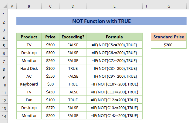
Example 6 –  Merge AND Function with TRUE Function

The AND function returns either TRUE or FALSE based on more than one condition.

Assuming that, you want to match the product and price with separate conditions e.g. product will be a TV and the price is greater than or equal to $500.

In such a situation, the formula will be:

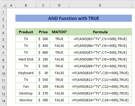
Example 7 – Combine COUNTIF with TRUE Function

The COUNTIF function counts the number of cells with criteria. You can use the function to count the number of TRUE in a cell range.

The formula would be:

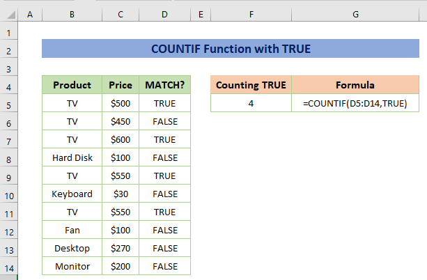
Example 8 – Finding Numerical Values

The ISNUMBER function checks the cell value whether it is a number or not. If the input is a number, the result will be shown as TRUE otherwise, FALSE.

The formula is:

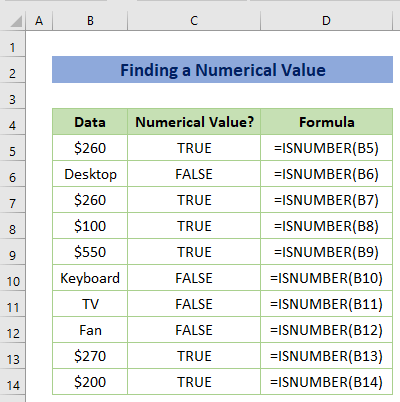
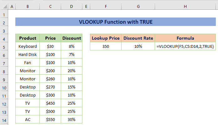
Example 9 – Merge VLOOKUP Function with TRUE Function (Approximate Match)

The VLOOKUP function finds the required value from a cell range based on the lookup value and types of the match i.e. TRUE is for an approximate (closest) match and FALSE is for an exact match.

For example, the products are given with price and discount rate. You have to find the discount rate if the price is $350. But such a price is not in the given table.

So, you have to find the closest discount rate for the price of $350.

For this, use the following formula:

The lookup price is $350, the cell range is C5:D14, 2 is the column index (as the price in the 2nd column) and TRUE is for an approximate match.

Note: While finding the approximate match, you must organize the value (cell range) from where you want to find the lookup value in ascending order. Otherwise, you’ll find inaccurate results.

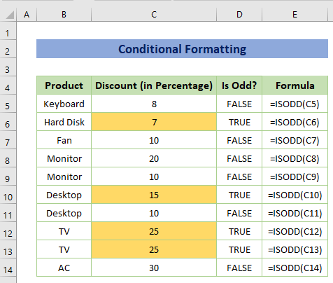
Example 10 – Conditional Formatting Using TRUE Function

To highlight the odd discount rate for better visualizations, you may use the Conditional Formatting toolbar from the Styles command bar.

Steps:

• Select the data and open a New Formatting Rule dialog box by clicking Home tab > Conditional Formatting > New Rules.

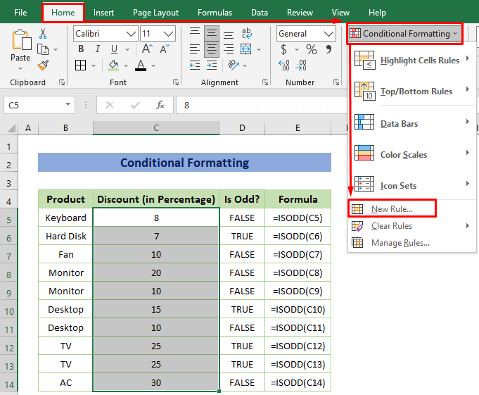
• Choose the option Use a formula to determine which cells to format, and insert the following formula for the odd number. Open the Format option to specify the highlighting color.

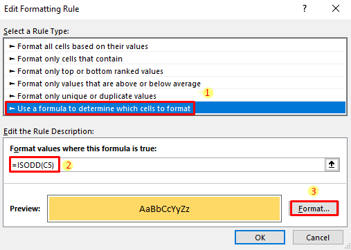
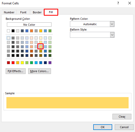
• Select your desired color from the Fill section. We chose the yellow color.

You’ll get the following output.

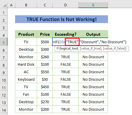
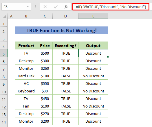
How to Fix When TRUE Function Is Not Working in Excel

In some cases, you may face problems while using the TRUE function. Have a  look at the sample dataset below. We have used the IF function to return ‘Discount’ for TRUE and ‘No Discount’ for FALSE. But, it’s only returning ‘No Discount’ for every price.

This is because we have used double quotes with TRUE and that is the mistake. We used double quotes for texts in the formula but here TRUE is not a text, it’s a function. The TRUE function works like the numerical value 1. It created this error as numerical value doesn’t need double quotes.

Solution:

• Remove the double quotes from the TRUE function and then the formula will work properly.

Things to Remember

• The output for TRUE() and TRUE are similar and we should not get confused between these two.
• Excel automatically returns either TRUE or FALSE for any type of logical expression.
• While computing, TRUE turns to 1 and FALSE turns to 0.

Download Practice Workbook

<< Go Back to Excel Functions | Learn Excel