While working in Excel, we often need to use the Text to Columns feature of Excel to split data into multiple columns. In the Text to Column option, we need to use a delimiter based on which we will separate the data. Carriage Return is one of the delimiters that are used in Excel. It basically creates a new line. Generally, in other software, we use the ENTER key. But in Excel, we need to use ALT + ENTER to create a new line in a cell. In this article, we will learn 3 easy steps to use the Text to Columns option with carriage return in Excel. So, let’s start the article and explore these steps.
How to Use Text to Columns Feature with Carriage Return in Excel: 3 Simple Steps
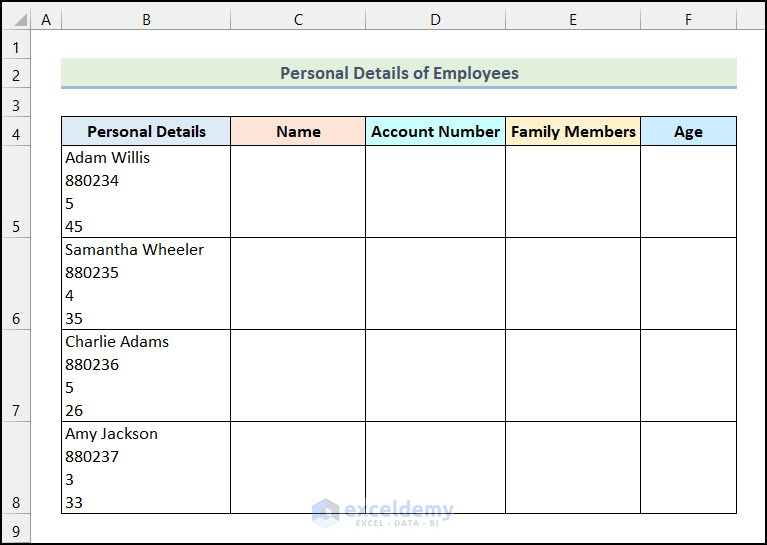
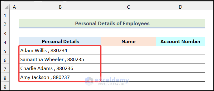
In this section of the article, we will learn 3 simple steps to use the Text to Columns option with carriage return in Excel. Let’s say, we have the Personal Details of Employees of a company as our dataset. In the dataset, we have all the details of an employee in a single cell. Our goal is to use the Text to Columns feature with carriage return to split them into separate cells.
Step 01: Select Data Type
In the first step, we will choose the data type of our texts. Let’s follow the steps mentioned below to do this.
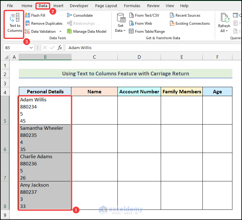
- Firstly, select the cells of the Personal Details column and go to the Data tab from Ribbon.
- After that, click on the Text to Columns option from the Data Tools group.
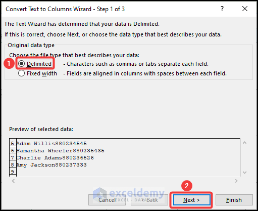
As a result, the Convert Text to Columns Wizard dialogue box will open on your worksheet.
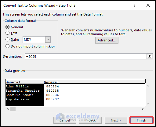
- Now, select the Delimited option in the Original data type field.
- Then click on Next.
Step 02: Choose the Delimiter
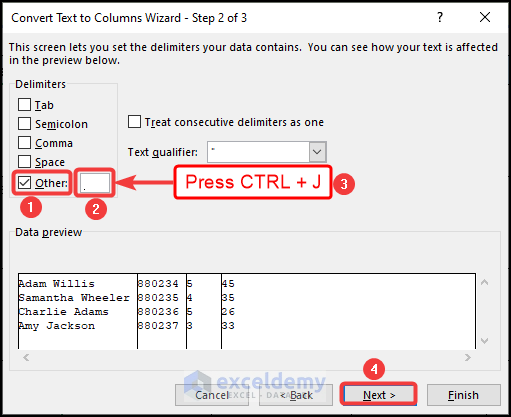
Now, we need to select a delimiter based on which we will split the cell contents into multiple columns.
- Firstly, check the box of the Other field and click on the blank box beside it.
- Then, use the keyboard shortcut CTRL + J.
- After that, click on Next.
Note: After using the keyboard shortcut, you will not see anything in the blank box beside the Other field. But you can see the Data Preview in the bottom section, and this is exactly what we are after.
Read More: How to Convert Column to Text with Delimiter in Excel
Step 03: Define the Destination Cell
In this step, we will define the destination cell where we want to display the data. If we don’t select any destination cell, Excel will replace the cell with the original data (cells of the Personal Details column). Let’s use the steps outlined below to select a destination cell.
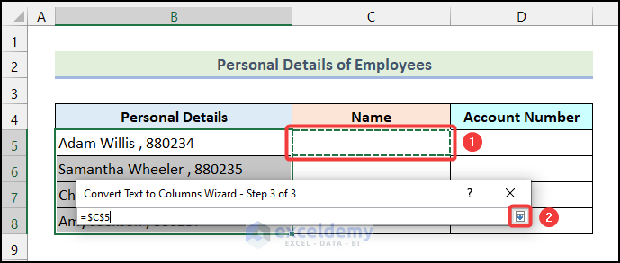
- Firstly, click on the marked area of the following picture.
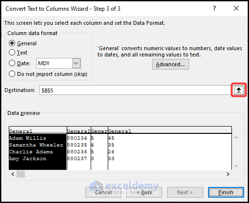
- After that, choose your preferred destination cell. Here, we selected cell C5 as our destination cell.
- Then, click on the marked portion of the image below.
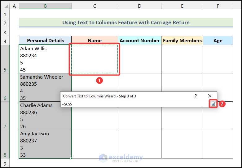
- Finally, click on Finish.

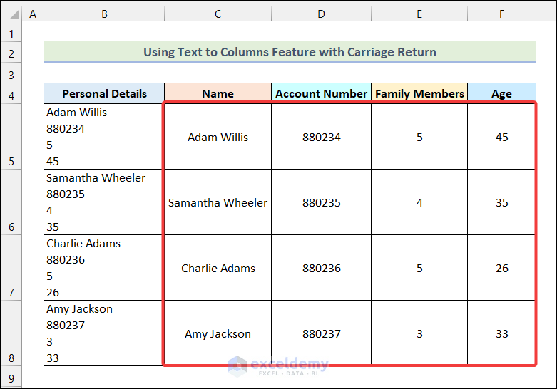
Consequently, your data will be split into 4 columns by using the Text to Column option of Excel with carriage return.
Application of Text to Columns Feature Using Word Delimiter in Excel
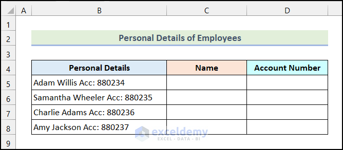
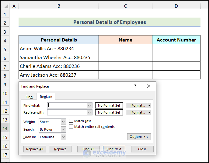
In this section of the article, we will discuss the procedure to use a word as a delimiter in the Text to Columns feature of Excel. Generally, we use space or a symbol that is common in all the cells to separate the data into different columns. Here, we will replace a common text with a symbol and use that as a delimiter. For instance, we have the Name and Account Number of some employees of a company in a single cell. Our goal is to separate Name and Account Number using a word as a delimiter.
Now, let’s follow the steps mentioned below.
Steps:
- Firstly, use the keyboard shortcut CTRL + H to open the Find and Replace dialogue box on your worksheet.
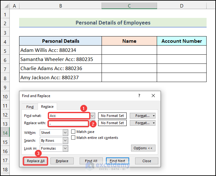
- Following that, type in “Acc:” in the Find what field as it is the common text in all cells.
- Then, type “,” in the Replace with field.
- Now, click on Replace All.
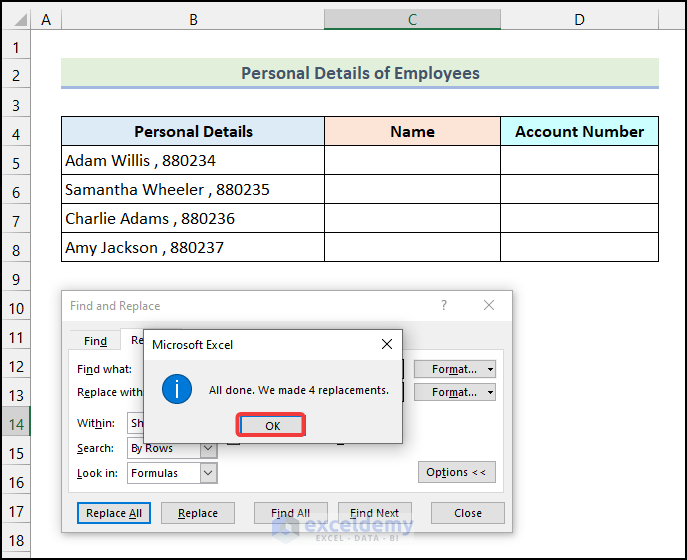
- After that, click on OK as marked in the following image.
- Next, click on Close in the Find and Replace dialogue box.
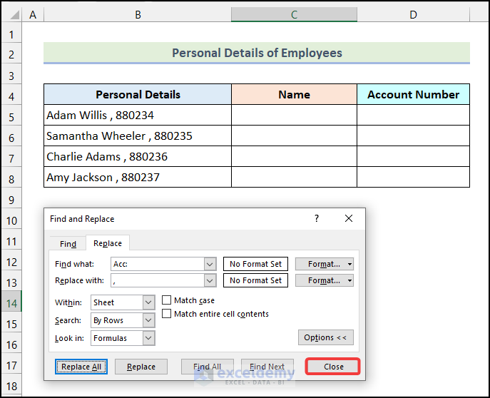
As a result, you will have the following output in the Personal Details column.
- Now, use the steps mentioned in Step 01 of the 1st method to obtain the following output.
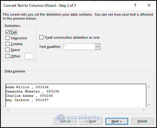
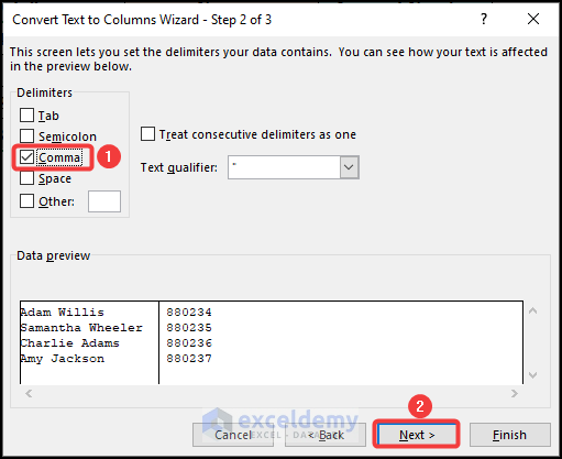
- Subsequently, check the box before Comma in the Delimiters section.
- Following that, click Next.
- Afterward, click on the marked area in the image below to select the destination cell.
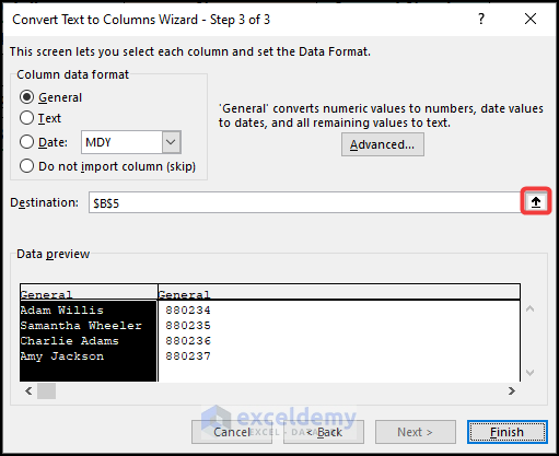
- Then, choose the destination cell. Here, we selected cell C5 as our destination cell.
- Next, click on the marked area of the following picture.
- Finally, click on Finish.
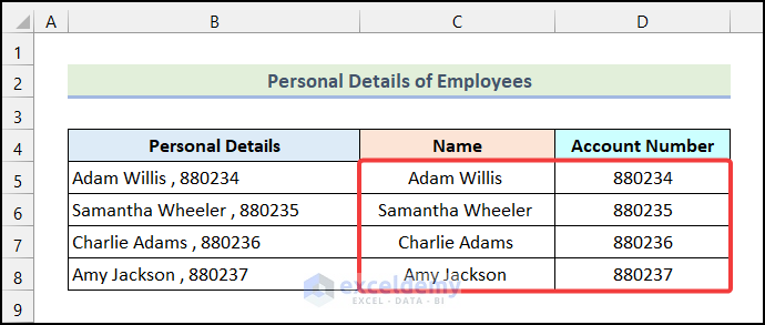
Consequently, you will have the following final outputs as demonstrated in the following picture.
Read More: How to Convert Text to Columns with Multiple Delimiters in Excel
How to Remove Carriage Return with Text to Columns in Excel
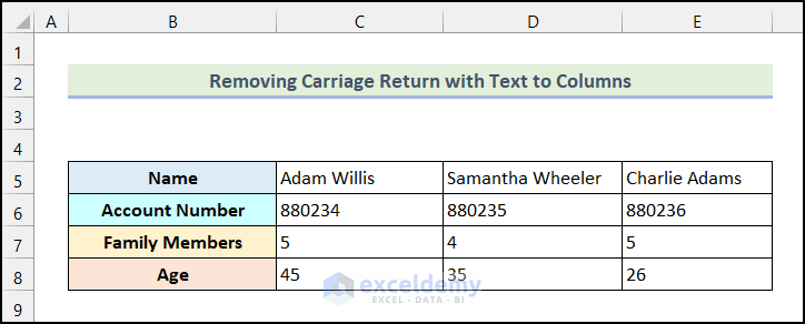
In Excel, we often encounter such datasets where all the data are cramped up using a carriage return, as demonstrated below. Although using a carriage return makes a dataset look clean, it is not suitable for doing any analysis. For this reason, we need to remove carriage return with Text to Columns in Excel. We are going to use the VBA Macro option of Excel to do this.

Consequently, you will have the following output in your worksheet, as demonstrated in the image below.
Read More: [Fixed!] Excel Text to Columns Is Deleting Data
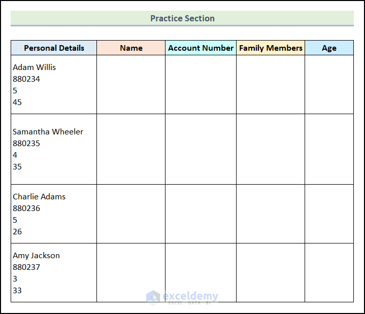
Practice Section
In the Excel Workbook, we have provided a Practice Section on the right side of the worksheet. Please practice it by yourself.
Download Practice Workbook
Conclusion
So, these are the most common & effective methods you can use anytime while working with your Excel datasheet to use text to column option with carriage return in Excel. If you have any questions, suggestions, or feedback related to this article you can comment below.
Related Articles
- How to Use Text to Columns in Excel for Date
- How to Convert Text to Columns Without Overwriting in Excel
- How to Split Text to Columns Automatically with Formula in Excel
- How to Undo Text to Columns in Excel
- Excel Text to Columns Not Working
- How to Use Line Break as Delimiter in Excel Text to Columns
- How to Convert Text to Columns in Excel with Multiple Spaces
<< Go Back to Excel Text to Columns | Splitting Text | Split in Excel | Learn Excel
Get FREE Advanced Excel Exercises with Solutions!
