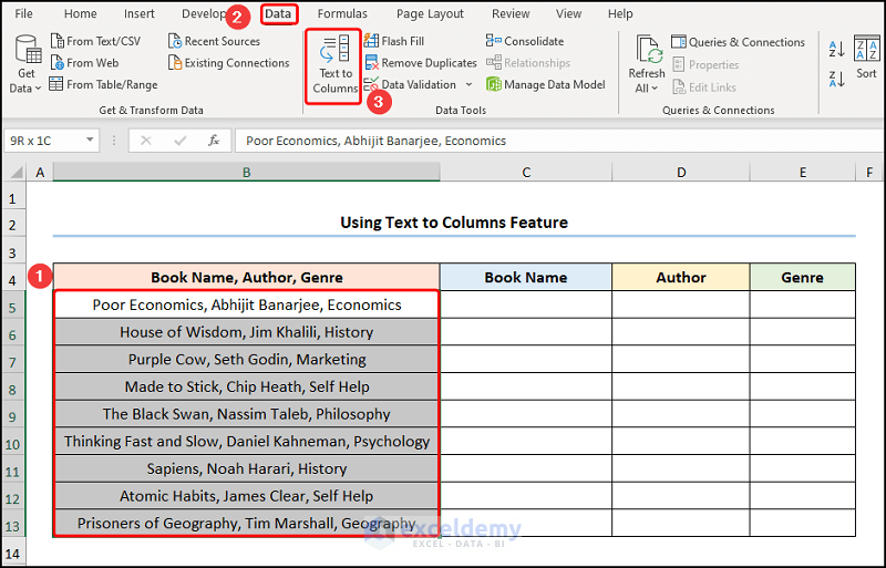
Our dataset, the List of Best Sellers, contains the Book Name, Author, and Genre columns. In this scenario, we want to split these columns into separate columns.

Method 1 – Using Text to Columns Feature
Steps:
- Select the B5:B13 cells >> go to the Data tab >> click the Text to Columns option.
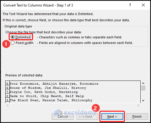
The Convert Text to Columns Wizard pops out.
- Choose the Delimited option >> Press Next.
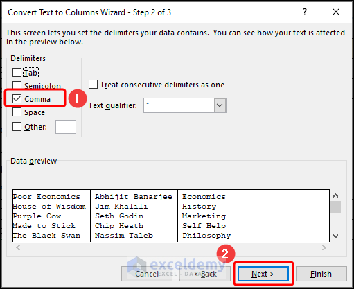
- Insert a check mark for the Comma delimiter >> Press Next.
- Enter a Destination cell according to your preference. Here it is cell C5 >> click Finish.
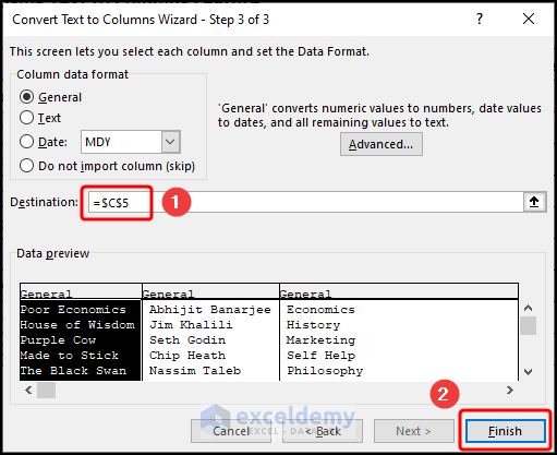
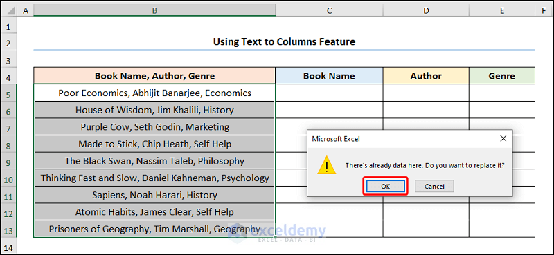
- A warning may appear. In this case, click OK.
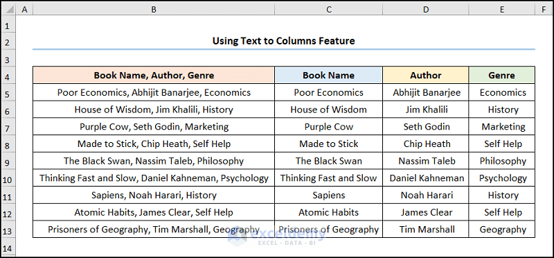
The final result should look like the screenshot given below.
Read More: How to Convert Column to Text with Delimiter in Excel
Method 2 – Utilizing TRIM, MID, SUBSTITUTE, REPT, and LEN Functions
Steps:
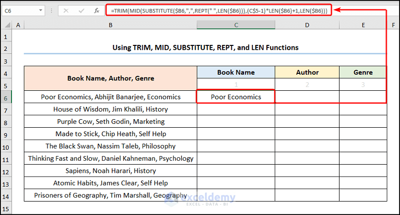
- Go to cell C6 >> enter the equation given below:
=TRIM(MID(SUBSTITUTE($B6,",",REPT(" ",LEN($B6))),(C$5-1)*LEN($B6)+1,LEN($B6)))
Here, the B6 and C5 cells refer to the Book Name, Author, Genre column, and the number 1.
Formula Breakdown:
- LEN($B6) → returns the number of characters in a string of text. Here, the B6 cell is the text argument that yields the value 43.
- Output → 43 ” “
- REPT(” “,LEN($B6)) → becomes
- REPT(” “,43) → repeats text a given number of times. Here, the ” “ is the text argument that refers to blank space, while the 43 is the number_times argument that instructs the function to insert 43 blank repeatedly.
- Output → ” “
- SUBSTITUTE($B6,”,”,REPT(” “,LEN($B6))) → replaces existing text with new text in a text string. Here, the B6 refers to the text argument while Next, the “,” represents the old_text argument, and the REPT(” “,LEN($B6)) points to the new_text argument which replaces the commas with blank spaces.
- Output → “Poor Economics Abhijit Banarjee Economics”
- MID(SUBSTITUTE($B6,”,”,REPT(” “,LEN($B6))),(C$5-1)*LEN($B6)+1,LEN($B6)) → returns the characters from the middle of a text string, given the starting position and length. Here, the SUBSTITUTE($B6,”,”,REPT(” “,LEN($B6))) cell is the text argument, (C$5-1)*LEN($B6)+1 is the start_num argument, and LEN($B6) is the num_chars argument such that the function returns the first character from the left side.
- Output → “Poor Economics “
- TRIM(MID(SUBSTITUTE($B6,”,”,REPT(” “,LEN($B6))),(C$5-1)*LEN($B6)+1,LEN($B6))) → becomes
- TRIM(“Poor Economics “) → removes all but single spaces from a text. Here, the “Poor Economics ” cell is the text argument and the function gets rid of excess spaces after the text.
- Output → “Poor Economics”
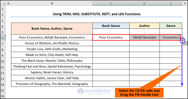
- Use the Fill Handle Tool to copy the formula across the rows.
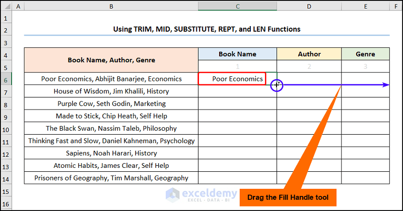
- Select the C6:E6 cells >> Drag the Fill Handle tool to apply the formula to the cells below.
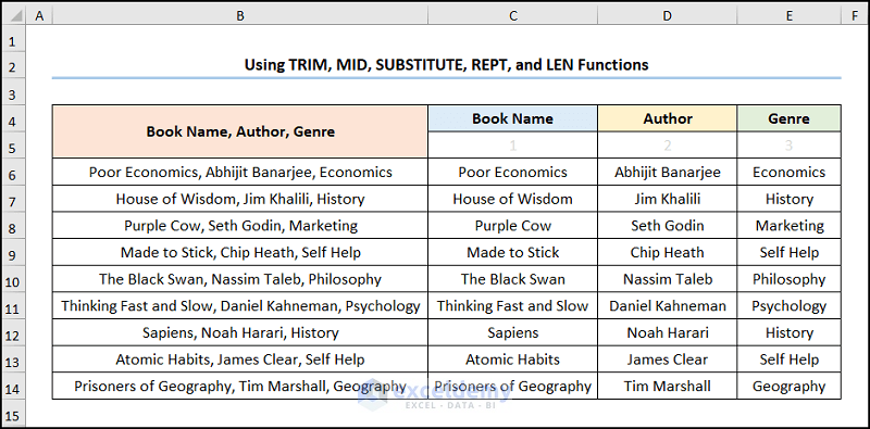
Your output should look like the picture shown below.
Read More: How to Convert Text to Columns in Excel with Multiple Spaces
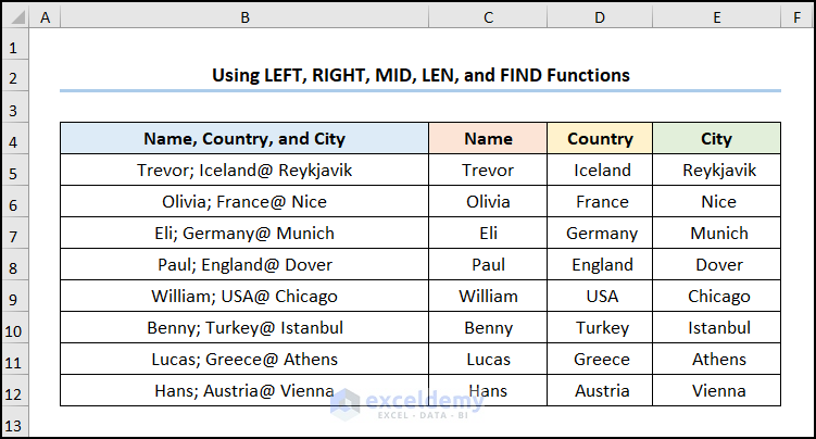
Method 3 – Combining LEFT, RIGHT, MID, LEN, and FIND Functions
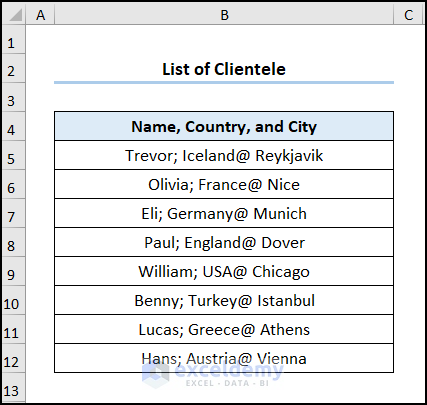
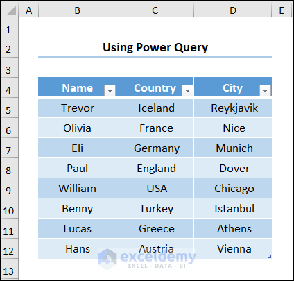
The List of Clientele dataset contains the Name, Country, and City columns with the texts separated by semicolons. Here, we want to split the Name, Country, and City into different columns.
Steps:
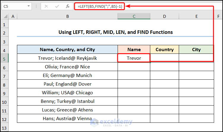
- Go to cell C5 >> insert the following expression into the Formula Bar:
=LEFT(B5,FIND(";",B5)-1)
In the above expression, the B5 cell represents the Name, Country, and City columns.
Formula Breakdown:
- FIND(“;”,B5) → returns the starting position of one text string within another text string. Here, “;” is the find_text argument while B5 is the within_text argument. Specifically, the FIND function returns the position of the semicolon(;) character in the string of text.
- Output → 7
- LEFT(B5,FIND(“;”,B5)-1) → becomes
- LEFT(B5,7) → returns the specified number of characters from the start of a string. Here, the B5 cell is the text argument, whereas 7 is the num_chars argument, so the function returns the 7 characters from the left side.
- Output → Trevor
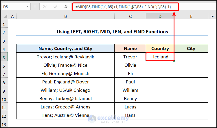
- Go to cell D5 >> type in the following expression:
=MID(B5,FIND(";",B5)+1,FIND("@",B5)-FIND(";",B5)-1)
Formula Explanation:
- FIND(“@”,B5)-FIND(“;”,B5)-1 → here, the FIND function returns the position of the semicolon(;) and the at the rate (“@”) characters within the string of text.
- 16 – 7 – 1 → 8
- FIND(“;”,B5)+1 → for example, the FIND function locates the the semicolon(;) characters within the string of text.
- 7 + 1 → 8
- MID(B5,FIND(“;”,B5)+1,FIND(“@”,B5)-FIND(“;”,B5)-1) → becomes
- MID(B5,8,8) → here, the B5 cell is the text argument, 8 is the start_num argument, and 8 is the num_chars argument such that the function returns the 8 characters after the first 8 characters.
- Output → Iceland
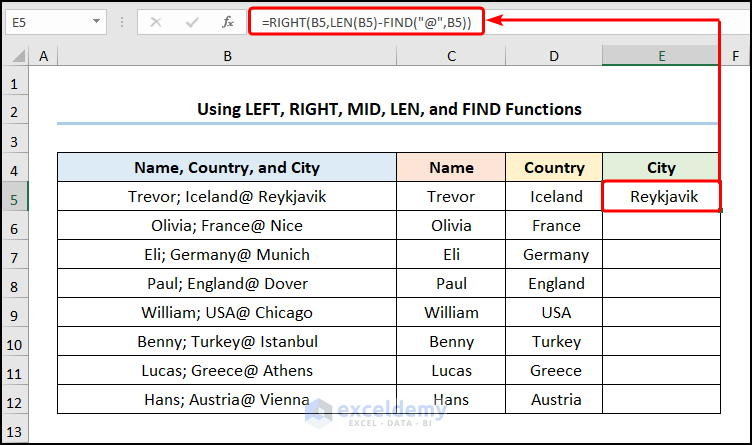
- Insert the formula below into cell E5:
=RIGHT(B5,LEN(B5)-FIND("@",B5))
How this Formula Works:
- LEN(B5)-FIND(“@”,B5) → the LEN function returns the length of the string in the B5 cell; in contrast, the FIND function returns the position of the at the rate (“@”) character.
- 26 – 16 → 10
- RIGHT(B5,LEN(B5)-FIND(“@”,B5)) → becomes
- RIGHT(B5,10) → returns the specified number of characters from the end of a string. Here, the B5 cell is the text argument, whereas 10 is the num_chars argument, so the function returns the 10 characters from the right side.
- Output → Reykjavik
The results should look like the screenshot below.
Read More: How to Split Text to Columns Automatically with Formula in Excel
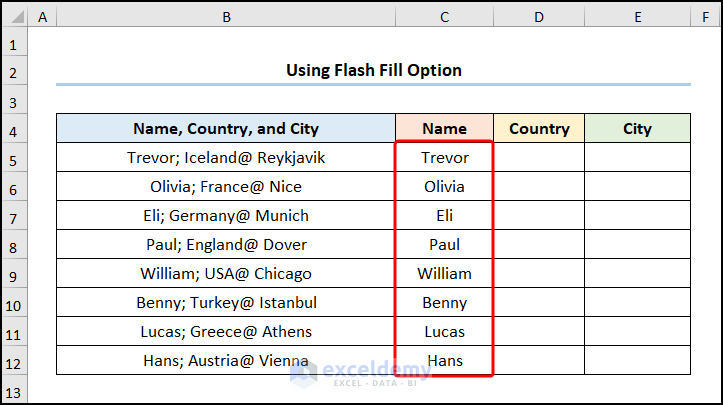
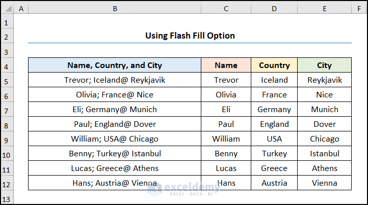
Method 4 – Employing Flash Fill
Steps:
- Type in the Name Trevor in cell C5 >> in the Home tab, click the Fill drop-down >> select the Flash Fill option.
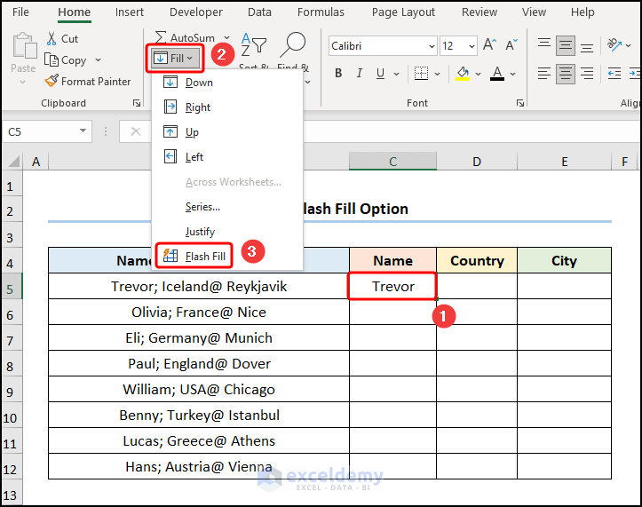
Excel will autofill the rest of the cell.
Apply the technique to the Country and City columns; the final output should look like the image below.
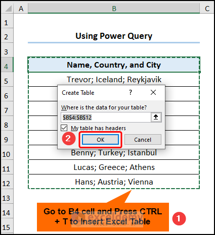
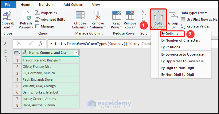
Method 5 – Using Power Query
Steps:
- Go to cell B4 >> press CTRL + T to insert an Excel Table >> press OK.
- Go to the Data tab >> click the From Table/Range option.
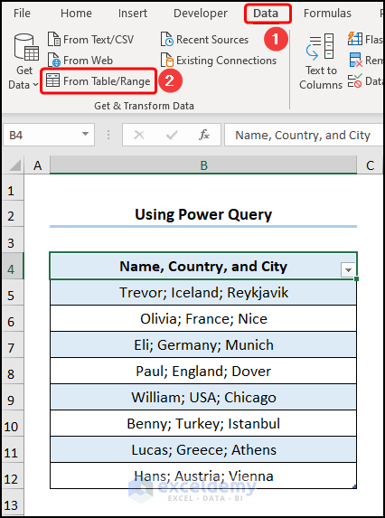
The Power Query Editor appears.
- Press the Split Column drop-down >> choose the By Delimiter option.
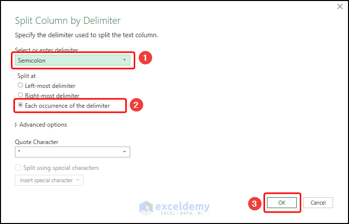
- Select the Semicolon option >> insert a check on Each occurrence of the delimiter option >> press OK.
- Double-click the column headers to rename them >> press the Close & Load option to exit the Power Query window.
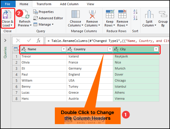
Completing all the steps should yield the following result.
Read More: How to Use Line Break as Delimiter in Excel Text to Columns
Method 6 – Applying VBA Code
Steps:
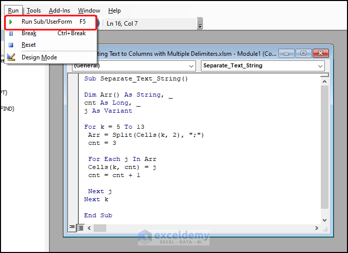
- Go to the Developer tab >> click the Visual Basic button.
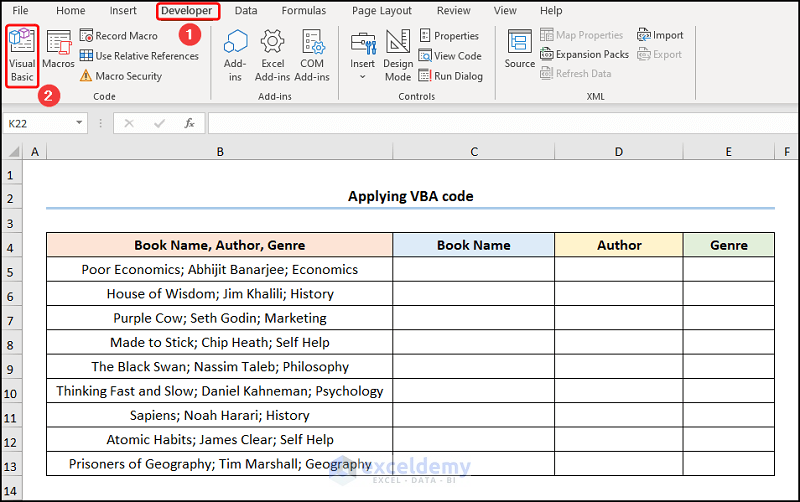
The Visual Basic Editor opens in a new window.
- Go to the Insert tab >> select Module.
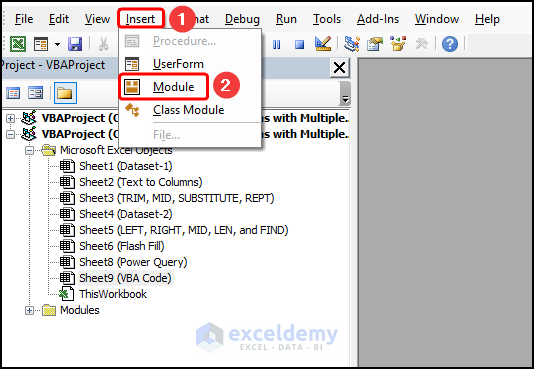
Copy the code from here and paste it into the window below:
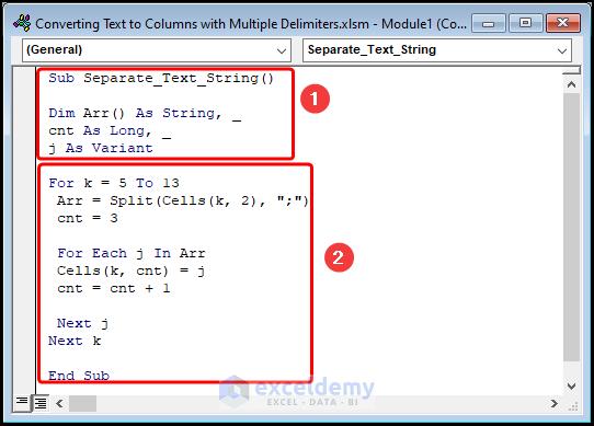
Sub Separate_Text_String()

Dim Arr() As String, _
cnt As Long, _
j As Variant

For k = 5 To 13
 Arr = Split(Cells(k, 2), ";")
 cnt = 3

 For Each j In Arr
 Cells(k, cnt) = j
 cnt = cnt + 1

 Next j
Next k

End Sub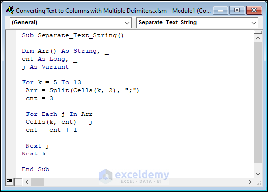
⚡ Code Breakdown:
Here, I will explain the VBA code used to convert text to columns with multiple delimiters. The code is divided into 2 steps.
- In the first portion, the sub-routine is given a name, here it is Separate_Text_String().
- Next, define the variables Arr, cnt, and j as String, Long, and Variant.
- In the second potion, use the For Loop through each cell and split the text delimited by semicolons.
- Now, in the code, the statement “For k = 5 To 13” represents the starting and ending row numbers of the data. Here, it is 5 to 13.
- Then, the “;” in the “Arr = Split(Cells(k, 2), “;”)” is the delimiter which you can change to a comma, pipe, etc., if you wish.
- Lastly, the “cnt = 3” indicates the third column number (Column C).
- Press Run or the F5 key.
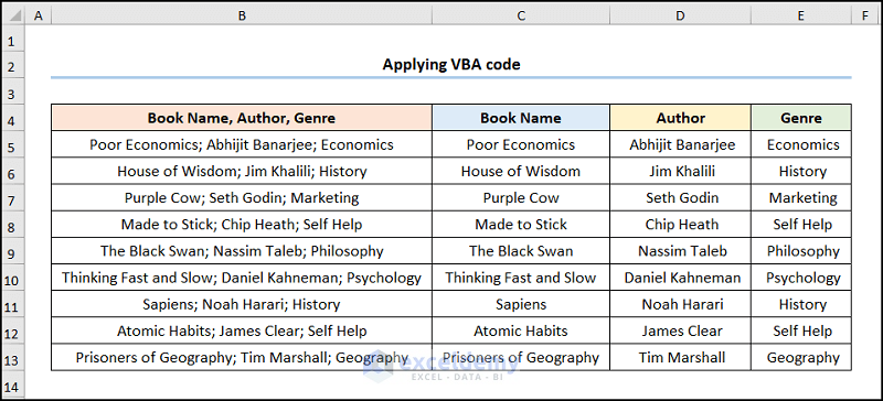
The results should appear in the screenshot given below.
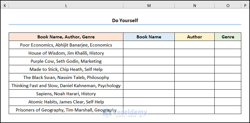
Practice Section
We have provided a practice section on the right side of each sheet so you can practice.
Download the Practice Workbook
Related Articles
- How to Convert Text to Columns Without Overwriting in Excel
- [Fixed!] Excel Text to Columns Is Deleting Data
- How to Undo Text to Columns in Excel
- Excel Text to Columns Not Working
<< Go Back to Splitting Text | Split in Excel | Learn Excel
Get FREE Advanced Excel Exercises with Solutions!
