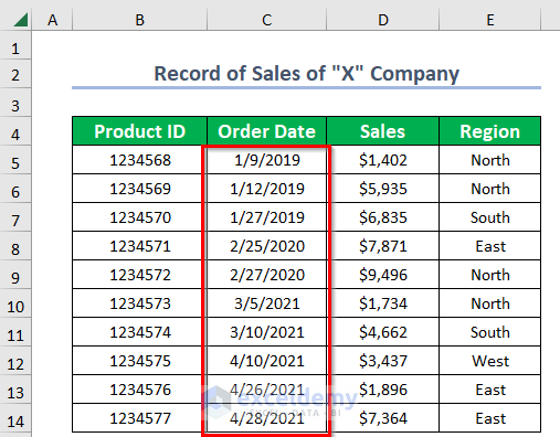
Let’s use a dataset with some sales and calculate total sales by month and year.

SUMIF by Month and Year: 7 Quick Ways
The dates in our starting dataset are formatted as mm-dd-yyyy. We’ll need to refer to them in formulas.
Method 1 – Use of SUMIFS Function to Do SUMIF by Month and Year
If you want to add the sales of January 2019 then you can use the SUMIFS function and the DATE function.
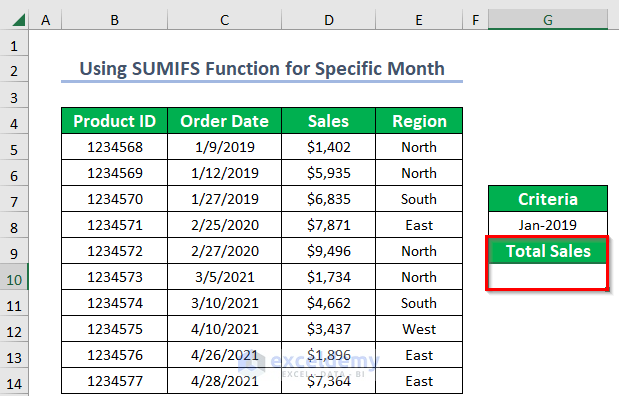
Steps:
- Select the output Cell G10.
- Copy the following formula:
=SUMIFS(D5:D14,C5:C14,">="&DATE(2019,1,1),C5:C14,"<="&DATE(2019,1,31))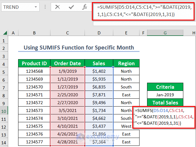
Formula Breakdown
- Here, D5:D14 is the range of Sales, and C5:C14 is the criteria range.
">="&DATE(2019,1,1)is the first criterion where DATE will return the first date of a month."<="&DATE(2019,1,31)is the second criterion where DATE will return the last date of a month.
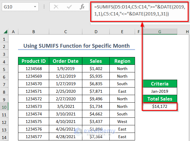
- Press Enter.
Result:
Method 2 – Using SUMIFS Function to Sum up Values Based on a Certain Period
You can get the sum of sales for a certain period like from January 2019 to February 2020.
Steps:
- Select the output Cell G10.
- Type the following formula and press Enter:
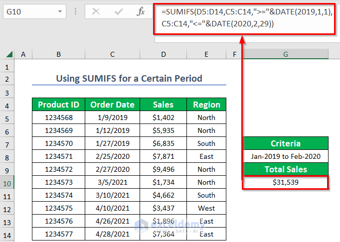
=SUMIFS(D5:D14,C5:C14,">="&DATE(2019,1,1),C5:C14,"<="&DATE(2020,2,29))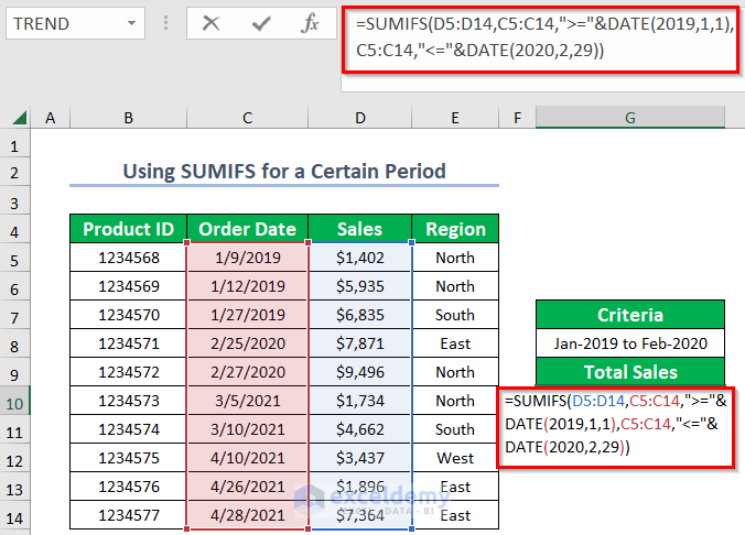
Formula Breakdown
- Here, D5:D14 is the range of Sales, and C5:C14 is the criteria range.
">="&DATE(2019,1,1)is the first criterion where DATE will return the first date of a period."<="&DATE(2020,2,29)is the second criterion where DATE will return the last date of a period.
Result:
Read More: How to Use SUMIF in Date Range and Month in Excel
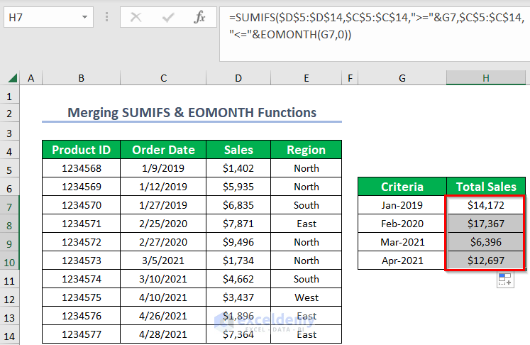
Method 3 – Combining SUMIFS & EOMONTH Functions
You can also get the sum of sales for a month or a year. Let’s put a few cells to determine which months to calculate the sales for.
Steps:
- Select the output Cell H7.
- Type the following formula:
=SUMIFS($D$5:$D$14,$C$5:$C$14,">="&G7,$C$5:$C$14,"<="&EOMONTH(G7,0))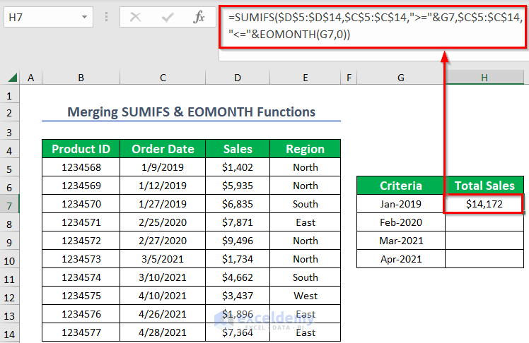
Formula Breakdown
- $D$5:$D$14 is the range of Sales, $C$5:$C$14 is the criteria range.
">="&G7is the first criterion where G7 is the first date of a month."<="&EOMONTH(G7,0)is the second criterion where EOMONTH will return the last date of a month.
- Press ENTER.
- Drag down the Fill Handle icon to copy the formula to the other cells.
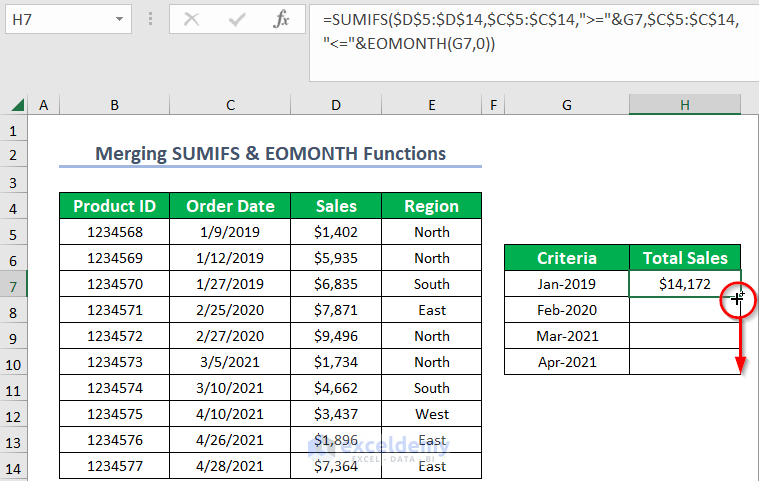
Result:
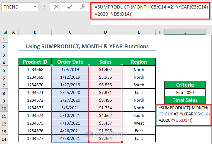
Method 4 – Merging SUMPRODUCT, MONTH & YEAR Functions to Add Values
Let’s get the sales for February 2020.
Steps:
- Select the output Cell G10.
- Type the following formula:
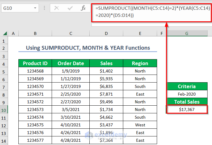
=SUMPRODUCT((MONTH(C5:C14)=2)*(YEAR(C5:C14)=2020)*(D5:D14))- Press Enter.
Formula Breakdown
- Here, D5:D14 is the range of Sales, and C5:C14 is the range of Dates.
- Then, MONTH(C5:C14) will return the months of the dates, and then it will be equal to 2 and which means February.
- Similarly, YEAR(C5:C14) will return the years of the dates, and then it will be equal to 2020.
Result:
Then, you will get the sum of sales for February of the year 2020.
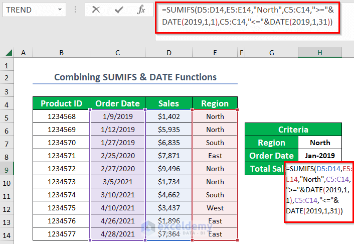
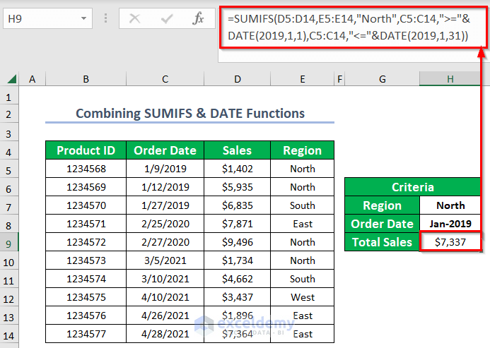
Method 5 – Summing up Values for a Month of a Year Based on Criteria
Steps:
- Select the output Cell H9.
- Type the following formula:
=SUMIFS(D5:D14,E5:E14,"North",C5:C14,">="&DATE(2019,1,1),C5:C14,"<="&DATE(2019,1,31))- Press Enter.
Formula Breakdown
- Here, D5:D14 is the range of Sales, E5:E14 is the first criteria range and North is the first criterion.
- Then, C5:C14 is both the second and third criteria range.
">="&DATE(2019,1,1)is the second criterion where DATE will return the first date of a period."<="&DATE(2019,1,31)is the third criterion where DATE will return the last date of a period.
Result:
Method 6 – Using SUM & IF Functions for a Month of a Year Based on Criteria
Let’s sum up the Sales for January of the year 2019 for criteria of the Region of North.
Steps:
- Select the output Cell H9.
- Type the following formula:
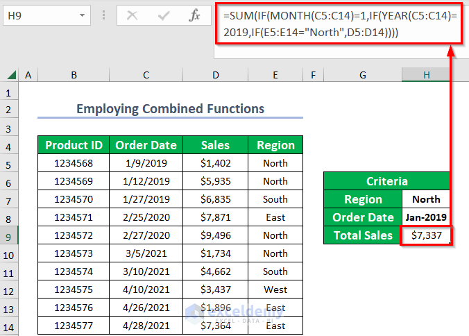
=SUM(IF(MONTH(C5:C14)=1,IF(YEAR(C5:C14)=2019,IF(E5:E14="North",D5:D14))))- Press Enter.
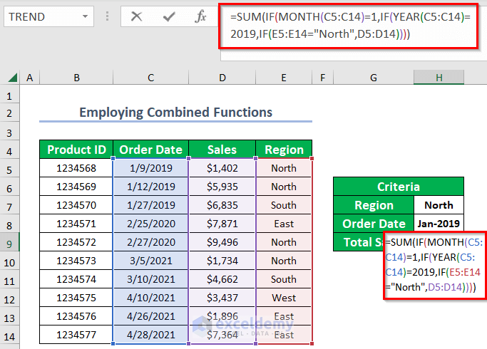
Result:
Read More: Sum Values Based on Date in Excel
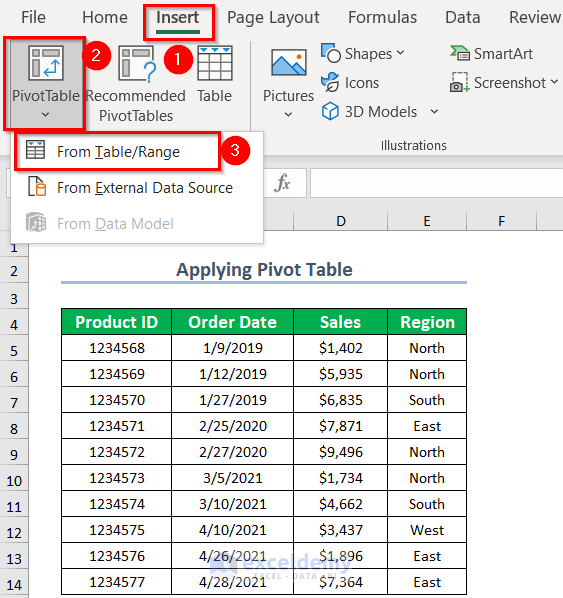
Method 7 – Using Pivot Table for Doing SUMIF by Month and Year
Steps:
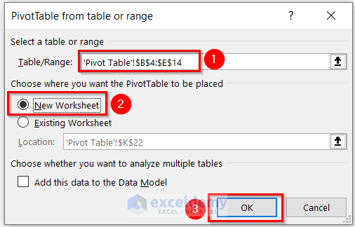
- Go to the Insert tab, select the PivotTable option, and choose From Table/Range.
As a result, PivotTable from table or range Dialog Box will pop up.
- Select the table/range as the entire dataset.
- Click on New Worksheet.
- Press OK.
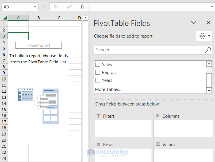
- A new sheet will appear where you have two portions named PivotTable1 and PivotTable Fields.
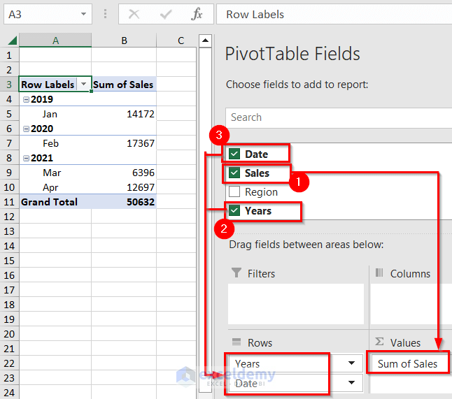
- Drag down Sales to the Values area.
- Drag Years and Date to the Rows area.
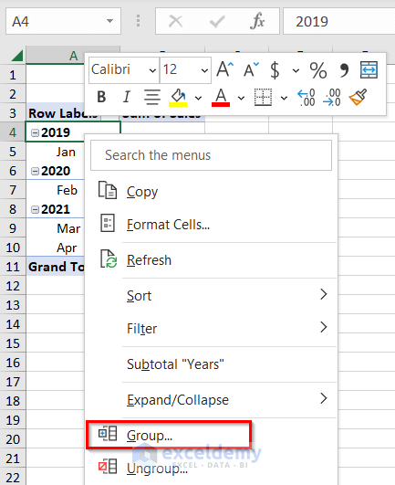
- Select any Cell of the Row Labels.
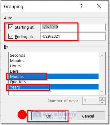
- Right-click and select Group. A Grouping Dialog Box will appear.
- Check the Starting at and Ending at the desired dates and mark the Months and Years option in the indicated area.
- Press OK.
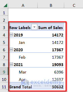
Result:
You will get the sum of sales for a month of a year as below.
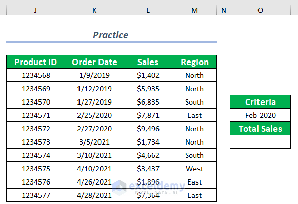
Practice Section
We have provided a practice worksheet for each method so you can tinker with the functions. Download it from the link below.
Download Practice Workbook
<< Go Back to SUMIF Date Range | Excel SUMIF Function | Excel Functions | Learn Excel
Get FREE Advanced Excel Exercises with Solutions!
