The IRR function is a financial function in Excel. It returns the Internal Rate of Return (IRR) for a given cash flow (the initial investment and a series of net income values) that occur at regular intervals. In this article, we will show you how to use the IRR function in Excel.
Introduction to The IRR Function
- Purpose
To calculate the internal rate of return.
- Syntax
=IRR(values, [guess])
- Arguments Description
| Argument | Required/ Optional | Description |
|---|---|---|
| values | Required | Arrays or range of cell references that contain values. |
| guess | Optional | Estimation of expected IRR. The default value is 0.1 or 10%. |
- Return Value
Calculated IRR as percentages.
How to Use IRR Function in Excel: 4 Examples
In this section, we will show you how to utilize the IRR function in Excel to calculate monthly cash flows in different ways.
1. Calculate Monthly Profit Flow by IRR Function
This is a solid example of the IRR function. Consider the following example. Here we will calculate the IRR of a Profit Flow that occurred in consecutive months.
Steps:
To calculate that, all we have to do is,
- Pass the range of cells inside the IRR function as a parameter and press Enter.
In our case, the formula is,
=IRR(C5:C11)Here,
C5:C11 = Array or range of cell references in Profit Flow column that contain values to calculate the IRR for.
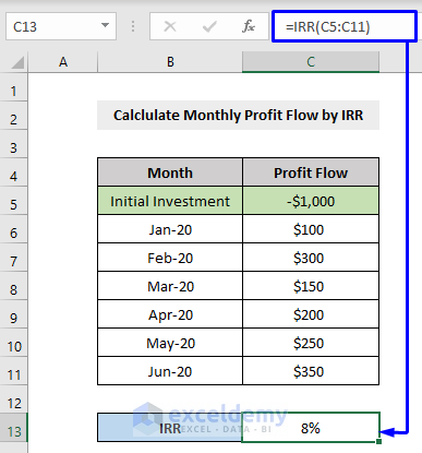
You will get the IRR value of your cash flow for sequential months.
2. Measure Monthly Profit Flow with Guess by IRR Function
Previously, we calculated the IRR only with the required argument, array value. But this time we will learn how to calculate monthly profit flow with Guess, which is an estimated value.
Steps:
To calculate profit flow with Guess,
- Write the generic IRR formula with the cell ranges as the first parameter, and
- Write the estimated value based on what you want your internal rate of the return value. We wanted an estimation of 20% of the IRR.
In our case, the formula is,
=IRR(C5:C11, 20%)Here,
C5:C11 = Array or range of cell references in Profit Flow column that contain values to calculate the IRR for.
20% = Guess value for the expected IRR.
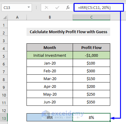
It will give you the IRR results with the estimated value that you provided.
3. Compare Between Monthly Profit Flows with the IRR Function
You can also compare cash flows between multiple projects. Look at the following example where we wanted to compare profit flows between multiple months in consecutive years.
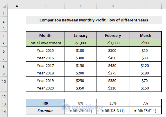
What we did here is, we calculated IRR for specific months in different years. For instance, to calculate the IRR for January,
- We pass all the cell ranges of column January inside the IRR
So the formula for January is,
=IRR(C5:C11)Here,
C5:C11 = Array or range of cell references in January column that contain values to calculate the IRR for.
- For February, the formula will be,
=IRR(D5:D11)As cell range D5:D11 holds the values for February
- Similarly, for March, the formula will be,
=IRR(E5:E11)As cell range E5:E11 holds the values for March; and so on.
Read More: How to Calculate IRR in Excel for Monthly Cash Flow
4. Calculate Compound Annual Growth Rate (CAGR) with IRR Function
Though Excel’s IRR function is designed to calculate the internal rate of return, you can also calculate the compound annual growth rate (CAGR) with it. To calculate that, all you have to do is, organize the data in a way that,
- Keep the first value (initial investment) as a negative number and the last value as a positive number.
- Replace the in-between cash flow values with zeros (to understand more, see the given picture below).
After that, simply write the regular IRR formula with the cell ranges as the parameter and press Enter.
In our case, the formula is,
=IRR(C5:C11)Here,
C5:C11 = Array or range of cell references in Revenue column that contain values to calculate the CAGR for.

It will produce the calculated internal rate of return for the CAGR of your data.
To check whether the value is truly correct or not, we run a mathematical CAGR formula,
=(end_value/-start_value)^(1/(number of periods-1)) -1
In our case, which shifted as,
=(C10/-C5)^(1/(6-1)) -1Here,
- C10 = end value
- C5 = start value
- 6 = number of periods
And we still got a similar result, hence the CAGR value produced by the Excel IRR function is correct.
Read More: How to Calculate IRR (Internal Rate of Return) in Excel
Things to Remember
- The first array argument, values, must contain at least one positive value and one negative value.
- If the calculation for IRR fails to assemble after 20 iterations, then the #NUM! value will occur.
- IRR is closely related to the Net Present Value (NPV) The rate of return calculated by the IRR is the discount rate while the NPV is equal to zero ($0).
Download Workbook
You can download the free practice Excel workbook from here.
Conclusion
This article explained in detail how to use the IRR function in Excel with examples. I hope this article has been very beneficial to you. Feel free to ask if you have any questions regarding the topic.
<< Go Back to Excel Functions | Learn Excel

