What Is Net Present Value?
If you have $1000 today, you can invest it in a business or buy a product today and sell it later, or at least you can deposit it with a bank that gives you interest for your deposits.
Say you have a trustable bank nearby, and they give 12% interest on deposits. You go to the bank and deposit $1000 with the bank at a 12% interest rate per year for the next 3 years.
Assume that you’re not withdrawing any money from the bank.
After 1 year, you will get:
$1000+ $1000 x 12% = $1000 (1+12%) = $1120So, $1120 after 1 year is the same as $1000 today.
After 2 years, you will get:
$1000 (1+12%) + $1000(1+12%)(12%) = $1000(1+12%)(1+12%) = $1000(1+12%)^2 = $1254.40So, $1254.40 after 2 years is the same as $1000 today.
In the same way, we can conclude that after 3 years, we shall get:
$1000(1+12%)^3 = $1404.93So, $1404.93 after 3 years is the same as $1000 today.
We can conclude an equation from the above discussion:
Future value of the money,
FV = PV((1+r)^n)Here,
- PV = Present value
- r = Interest rate/year
- n = Number of years
Reversely, we can calculate the present value of the money with this equation:
PV = FV/((1+r)^n)What Is the Internal Rate of Return (IRR)?
IRR is the interest rate that balances your initial investment and future cash flows.
Let’s start with an investment proposal you got:
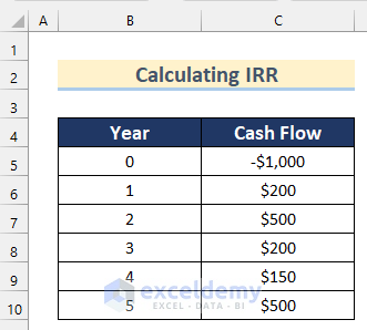
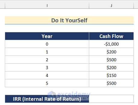
Sam is your friend who comes to you with an investment proposal. You are proposing to invest $1000, and these are the cash flows you can expect from the investment over the next 5 years.
There is a bank nearby your place, and you trust this bank. This bank provides 12% yearly interest on a deposit. Or you can invest your money in a government savings bond with a 10% interest rate/per year. A government bond is more secure than depositing with a bank. So, you have three options to invest your $1000:
- You can invest in your friend Sam’s project
- You can deposit the amount in your preferred bank that provides a 12% interest rate per year
- Or you can buy a government bond and enjoy a more secure income
What will you do? To make a better decision, you must first know the internal rate of return on your investment with Sam’s project.
Let’s calculate the IRR of these cash flows. There are several cash flow scenarios (regular, discrete, monthly, etc.), so your approach will also be different when you calculate IRR.
Method 1 – Using the IRR Function to Calculate IRR
Steps:
- Select cell C12 and insert the following formula:
=IRR(C5:C10)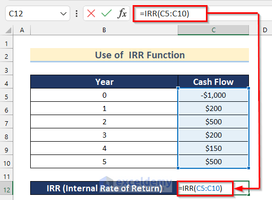
As the values argument, we have passed this cell range, C5:C10. The values must contain at least one negative value and one positive value. Otherwise, the IRR function will provide an #NUM! error value.
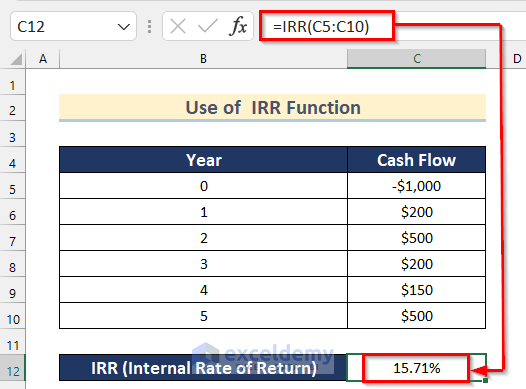
- Press ENTER to get the value of IRR.
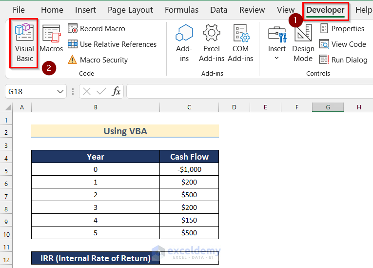
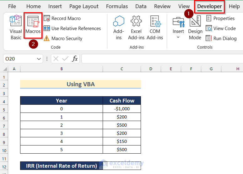
Method 2 – Applying VBA to Calculate IRR in Excel
Steps:
- Go to the Developer tab >> click on Visual Basic.
- The Microsoft Visual Basic for Application box will open.
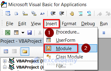
- Click on Insert >> Select Module.
- Enter the following code in your Module:
Sub Calculate_IRR()
Static CashFlow(6) As Double
CashFlow(0) = -1000
CashFlow(1) = 200
CashFlow(2) = 500
CashFlow(3) = 200
CashFlow(4) = 150
CashFlow(5) = 500
Cells(12, 3) = IRR(CashFlow())
End Sub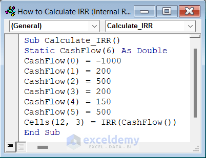
Code Breakdown
- Firstly, I created a subprocedure called Calculate_IRR().
- Then, I declared a Static array and named it CashFlow, where the size and type are Double.
- After that, I inserted 6 values of CashFlow as -1000, 200, 500, 200, 150, and 500, as given in our dataset.
- Finally, I used the VBA IRR function, inserting these CashFlow array values into the function and assigning this value to Cell (12,3).
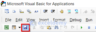
- Click on the Save button and go back to your worksheet.
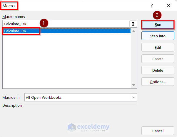
- Go to the Developer tab >> click on Macros.
Now, the Macros box will appear.
- Select Calculate_IRR.
- Click on Run.
- You will get your IRR value in decimal.
- To change the number format, go to the Home tab >> click on Number Format >> select Percentage.
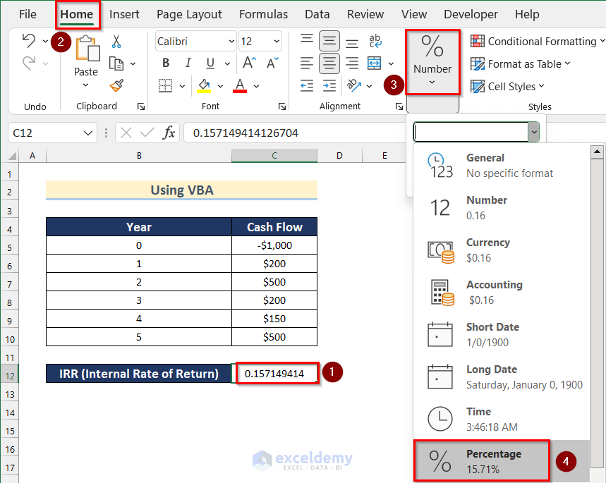
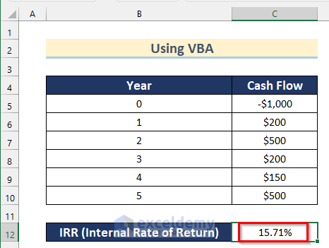
- You will get the value of IRR in percentage using VBA.
Method 3 – Manually Calculating IRR from Net Present Value in Excel
Steps:
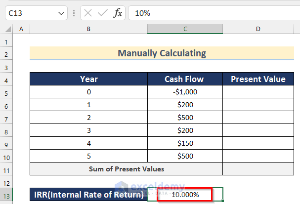
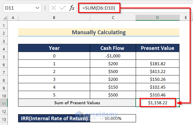
- Insert any value of your choice in Cell C13 as IRR. Here, I will insert 10%.
- Select cell D6 and insert the following formula:
=C6/(1+$C$13)^B6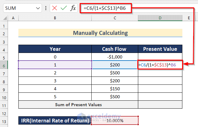
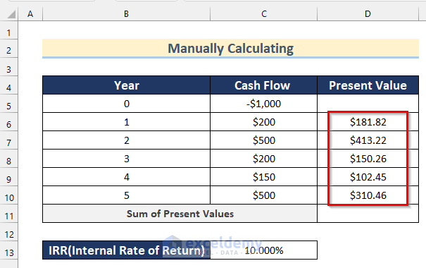
- Press ENTER and drag down the Fill Handle tool to AutoFill the formula for the rest of the cells.
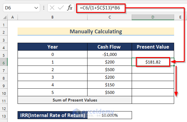
- You will get all the values of the Present Value.
- Select cell D11 and insert the following formula:
=SUM(D6:D10)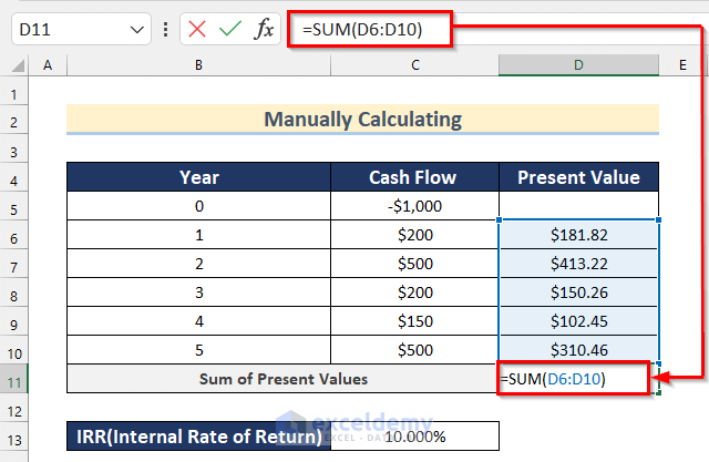
Here, in the SUM Function, we added all the Present Values in Cell range D6:D10.
- Press ENTER to get the total present value.
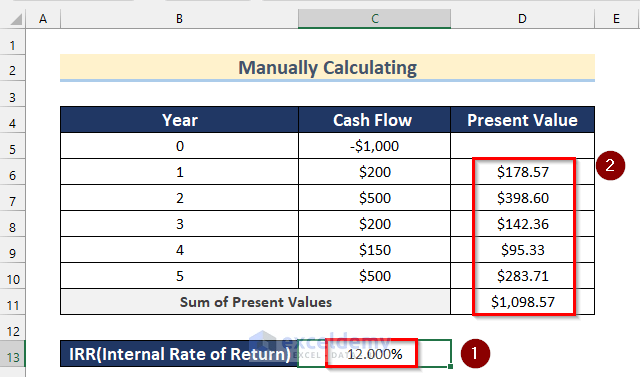
- In cell C13, you have to change the value manually to get a nearby value that makes the total present values equal to 1000.
- We change the value to 12%. Now, you see the total present value is $1098.57.
- Change the value to, say, 16%. The value in cell C8 is $993.03.
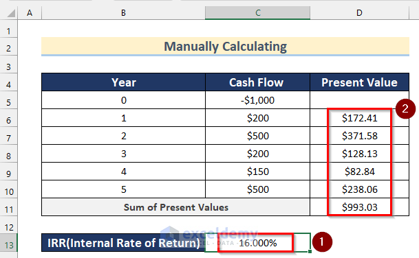
This is the manual way. It is not tough, but getting a very close value from this method will take time. You can also try this method on paper, but it might take a whole day to find the internal rate of return for some future cash flows.
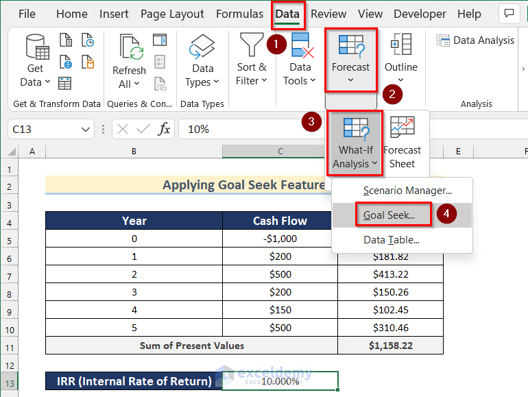
Method 4 – Applying the Goal Seek Feature to Calculate IRR in Excel
Steps:
- Go through the steps shown in Method 3 to prepare the dataset to use the Goal Seek feature.
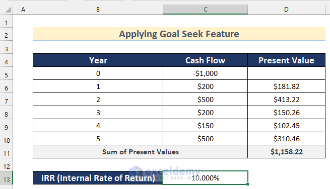
- Go to the Data tab >> click on Forecast >> click on What-If Analysis >> select Goal Seek.
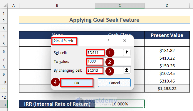
- The Goal Seek box will appear.
- Insert in cell D11 (sum of all future cash flows) as Set cell, 1000 (equal to initial investment) as To value, and Cell C13 (Internal Rate of Return) as By changing cell.
- Press OK.
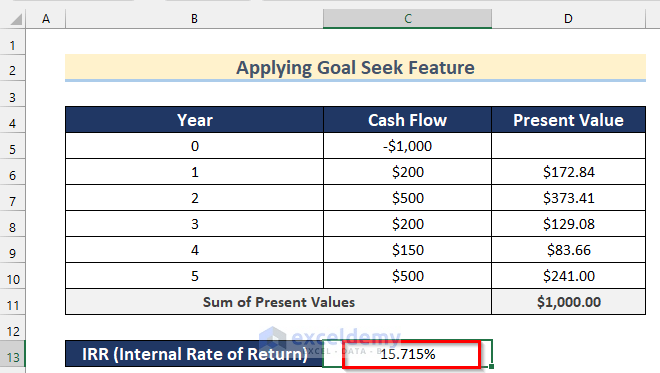
- The Excel Goal Seek feature does the iterations and comes up with a value that meets all the criteria. Here, you will get 15.715% as an IRR value that meets all the criteria and get the same internal rate of return as we got using Excel’s IRR function.
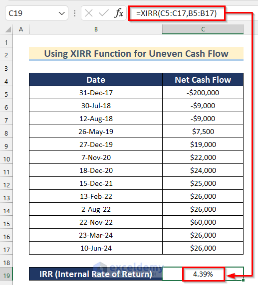
Method 5 – Using the XIRR Function to Calculate IRR for Uneven Cash Flow
Steps:
- Select cell C19 and insert the following formula:
=XIRR(C5:C17,B5:B17)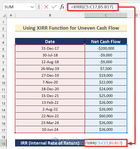
In the XIRR function, I inserted Cell range C5:C17 as values and Cell range B5:B17 as dates.
- Press ENTER to get the value of IRR.
Method 6 – Calculating IRR for Monthly Cash Flow in Excel
Steps:
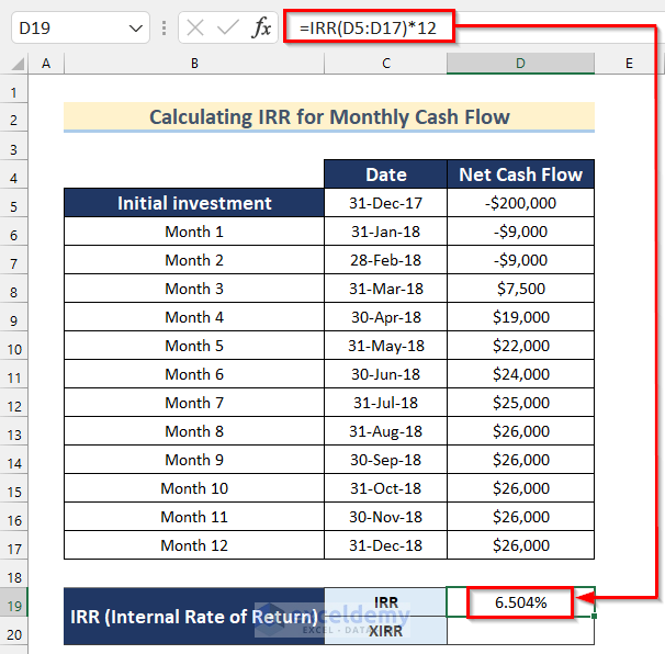
- Select cell D19 and insert the following formula:
=IRR(D5:D17)*12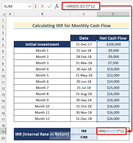
In the IRR function, I inserted Cell range D5:D17 as values and multiplied this by 12.
- Press ENTER to get the value of IRR using the IRR function.
- Select cell D20 and insert the following formula:
=XIRR(D5:D17,C5:C17)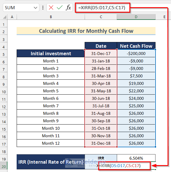
In the XIRR function, I inserted Cell range D5:D17 as values and Cell range C5:C17 as dates.
- Press ENTER to get the value of IRR using the XIRR function.
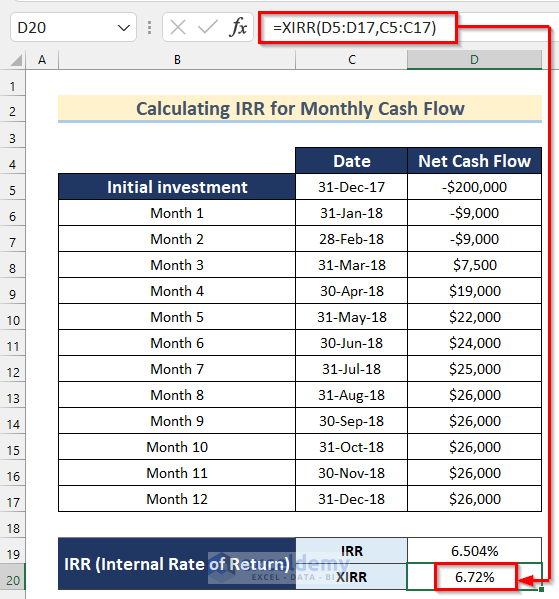
You see, there is a difference between the values.
Note: If you use the IRR function to calculate the internal rate of return for monthly cash flows, you need to multiply the IRR value by 12, as IRR calculates the monthly rate of return, not yearly.
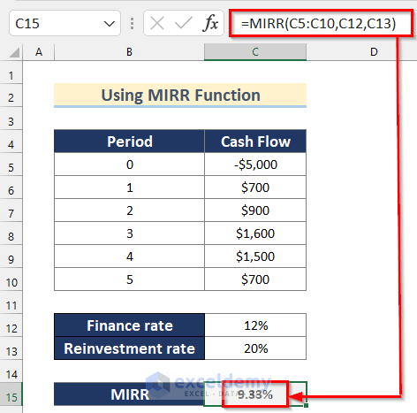
Method 7 – Using the MIRR Function to Calculate Modified IRR in Excel
Steps:
- Select cell C15 and insert the following formula:
=MIRR(C5:C10,C12,C13)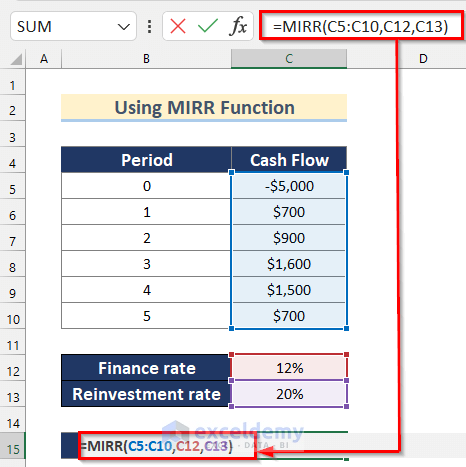
In the MIRR function, I inserted values for cell range C5:C10, cell C12 as finance_rate, and cell C13 as reinvest_rate.
- Press ENTER to get the value of IRR.
Method 8 – Calculating IRR for Real Estate in Excel
Steps:
- Select cell C8 and insert the following formula:
=SUM(C5:C7)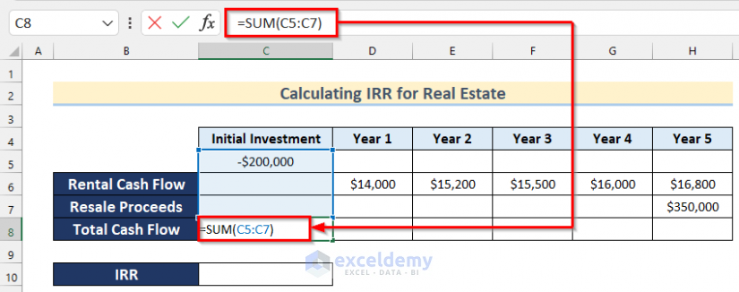
- Press ENTER and drag right the Fill Handle tool to AutoFill the formula for the rest of the cells.
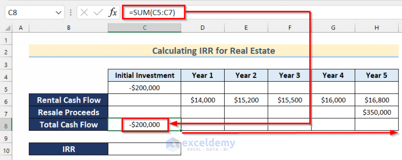
In the SUM function, I have added all the values of the cell range C5:C7.
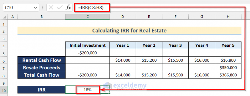
- Select cell C10 and insert the following formula:
=IRR(C8:H8)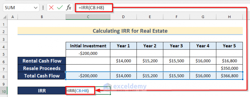
In the IRR function, I inserted cell range C8:H8 as values.
- Press ENTER to get the value of IRR for this real estate company.
What Is Good IRR?
It is a very tough question to answer. Usually, the IRR value is compared with a fixed value, such as a bank interest rate or a government bond rate, as you can earn these incomes idly without doing anything and risking anything. IRR has also compared the project to the project basis.
The following image shows data from two projects and their expected revenue over the next five years.
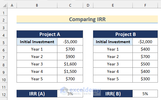
After calculating the IRR of these projects, it seems that Project B would have more potential for the company.
Practice Section
In this section, we provide you with the dataset to practice these methods on your own.
Download the Practice Workbook
<< Go Back to Excel Functions | Learn Excel
Get FREE Advanced Excel Exercises with Solutions!

Kawser
Very understandable and effective article regarding Internal Rate of Return ( IRR). I have one point to complain on comparison IRR and XIRR. It seems that as IRR is a monthly rate and to compute it annually we must use a compound form. as (IRR ^12) and not multiplied. Doing so we have IRR = 0,542% monthly – and ( 1,00542^12) we get 6,70 % – quite the same om XIRR ( 6.72%).
Looking for a prompt reply.
Regards
Hi Colvis.
We are very sorry for not reaching out to you promptly. But the annual IRR is calculated by multiplying the monthly IRR by 12. In that case, we get an annual IRR value of 6.504%. The value of IRR from the IRR formula and the XIRR formula should not be the same for irregular cash flows. And these values reflect that.
Hi – I am always confused with IRR as I say to myself (ok, it is used to give us an indication that Present Investment = Future Cash Flows) but how do we actually apply this in the “real world”. Can you please give me further insight with regard to your last example comparing Project A to Project B. Finally, is IRR of A (3%) and B (5%) of any relevance to the comparison of the “profitability” of these projects? In order to do so, wouldn’t we need to introduce WACC?
Thank you in advance for coming back to me on this.
Regards,
Romesh
Hi Romesh.
IRR is not the sole measure of comparing profitability. It is just one of the many parameters you can use to compare two paths of investment.
This is a wonderful articles . Great many thanks
We are glad that this helped.