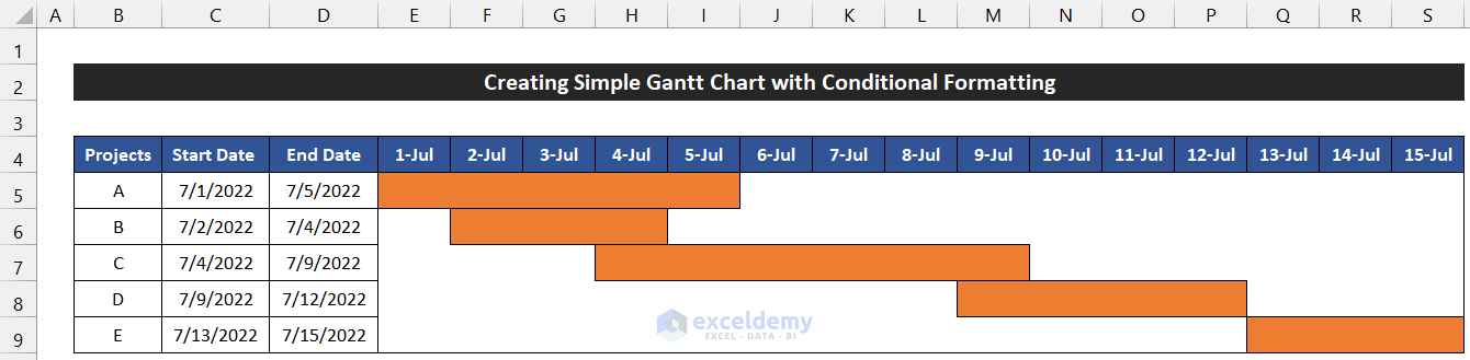
Example 1 – Creating Simple Gantt Chart with Conditional Formatting
Steps:
- Enter the dates 1 July-15 July in the range of cells E4:S4.
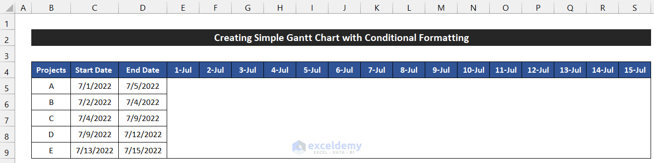
- Select the range of cells E5:S9.
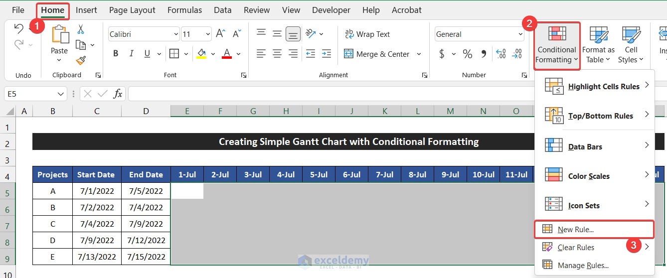
- Go to the Home tab, in the Styles group, click on the drop-down arrow of Conditional Formatting.
- Select New Rule.
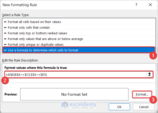
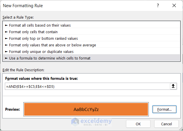
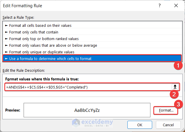
- New Formatting Rule box will open.
- Choose the Use a formula to determine which cells to format option.
- Enter the following formula,.
=AND(E$4>=$C5,E$4<=$D5)
- Click on Format.
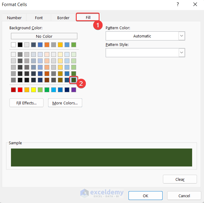
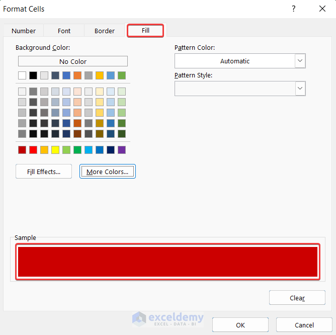
- The Format Cells box will open.
- In the Fill tab, choose your desired background color. For our chart, we chose Orange, Accent 2.
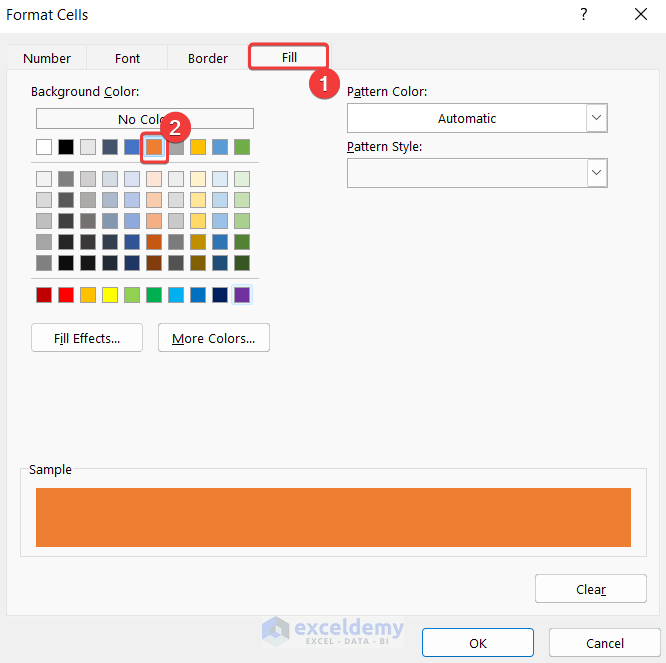
- Click OK to close the Format Cells dialog box.
- Click OK to close the New Formatting Rule dialog box.
- The Gantt chart for multiple projects is ready.
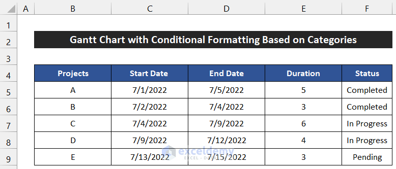
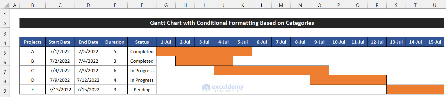
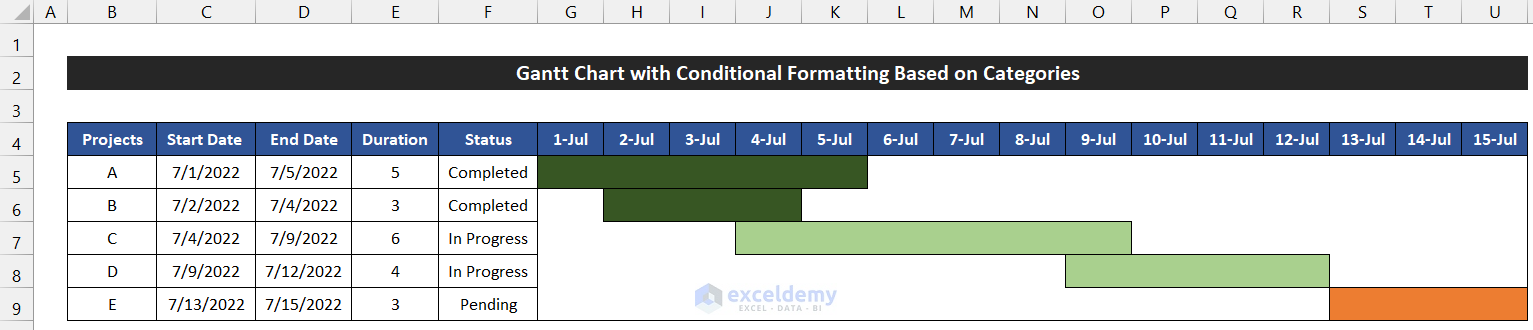
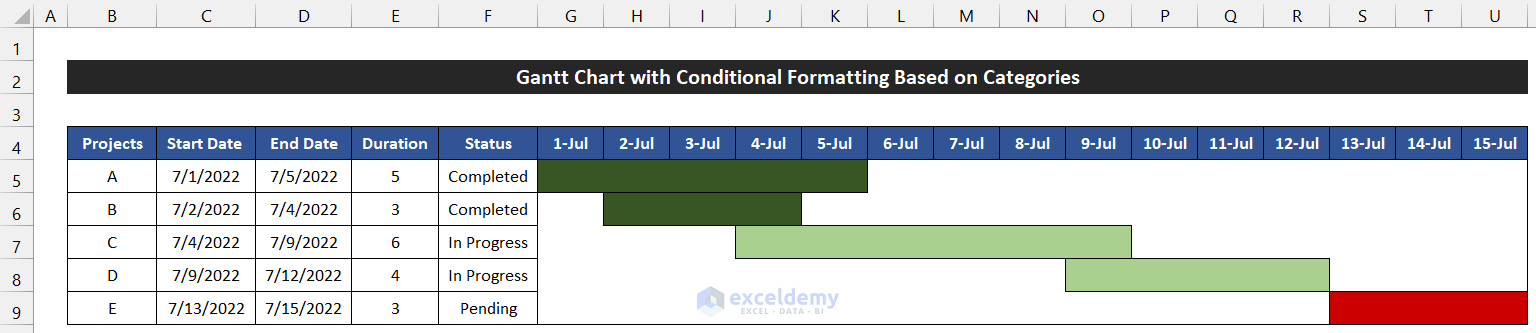
Example 2 – Gantt Chart with Conditional Formatting Based on Categories
Steps:
- To estimate the duration of the projects.
- Enter the following formula into cell E5.
=DAYS(D5,C5)+1
- Press Enter.
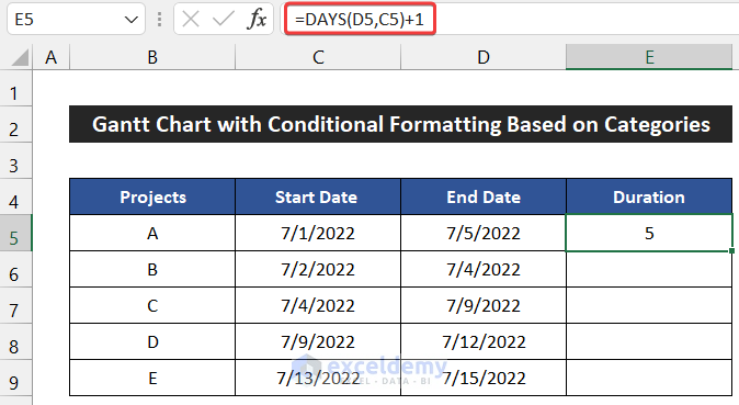
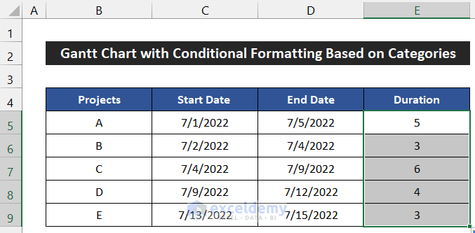
- Double-click on the Fill Handle icon to fill the formula till cell E9.
- Enter the Status of our projects in the range of cells F5:F9. We have chosen three different statuses for our projects Completed, In Progress and Pending.
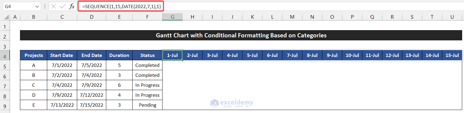
- To get the first 15 days date of our desired month, enter the following formula in cell G4.
=SEQUENCE(1,15,DATE(2022,7,1),1)
Breakdown of the Formula
DATE(2022,7,1): This function returns the first date of the month of July, 7/1/2022.
SEQUENCE(1,15,DATE(2022,7,1),1): This formula get the first starting point from the DATE function. Then, the function returns the other 15 dates in a row and 15 columns with unit intervals.
- Press Enter.
- You will get all the dates from 1 July-15 July in the range of cells G4:U4.
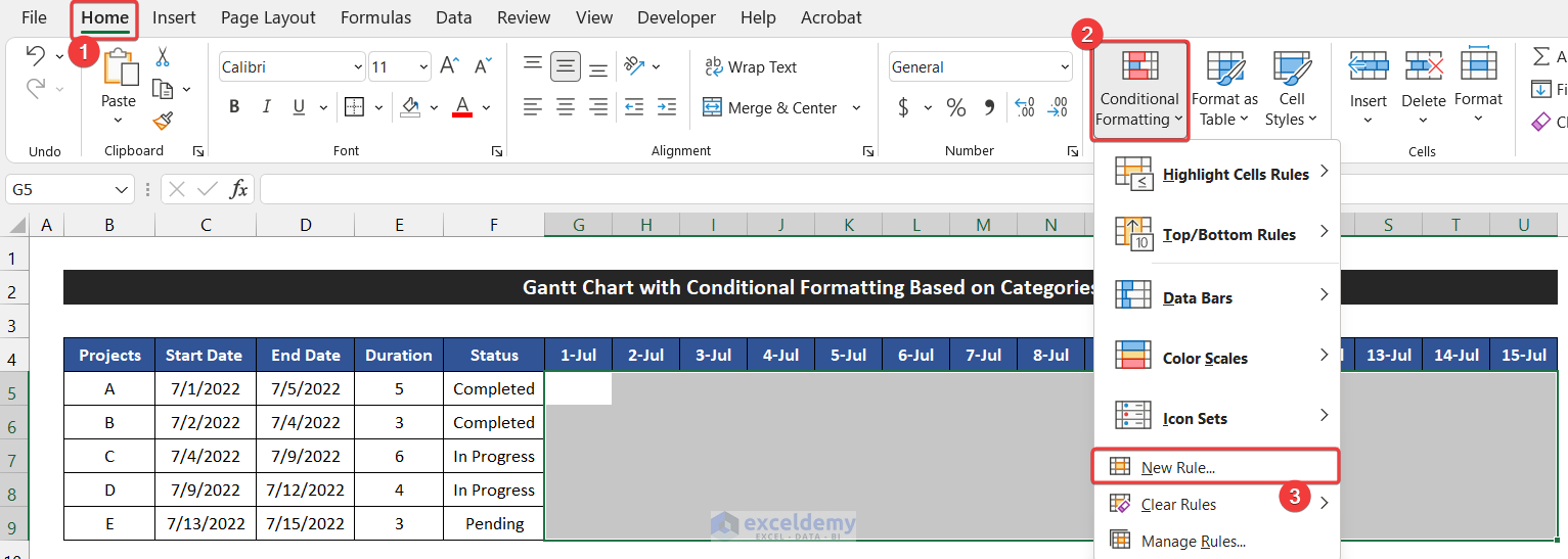
- Apply the general conditional formatting.
- Select the range of cells G5:U9.
- Go to the Home tab, in the Styles group, click on the drop-down arrow of the Conditional Formatting.
- Choose New Rule.
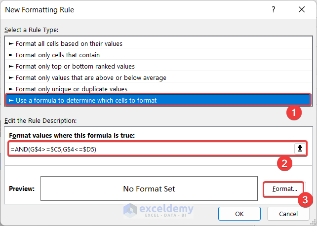
- The New Formatting Rule box will open.
- Choose the Use a formula to determine which cells to format option.
- Enter the following formula.
=AND(G$4>=$C5,G$4<=$D5)
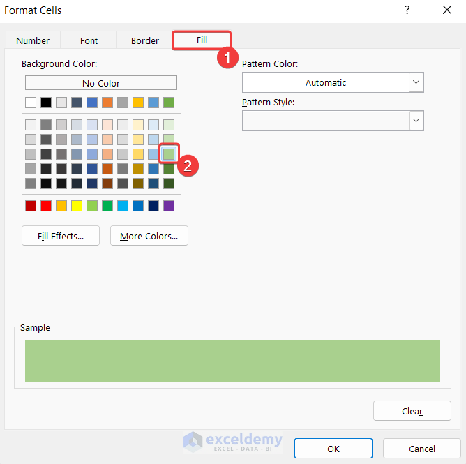
- Click on Format.
- The Format Cells box will open.
- In the Fill tab, choose your background color. We chose Orange, Accent 2.
- Click OK to close the Format Cells dialog box.
- Click OK to close the New Formatting Rule dialog box.
- Apply the cell formatting based on our category.
- Select the range of cells G5:U9 and open the New Formatting Rule dialog box.
- Enter the following formula:
=AND(G$4>=$C5,G$4<=$D5,$F5="Completed")
- Choose a different color for this category. We chose Green, Accent 6, Darker 50%.
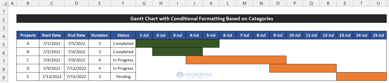
- The “Completed” projects show the selected color.
- Enter the following formula for the In Progress criteria,
=AND(G$4>=$C5,G$4<=$D5,$F5="In Progress")
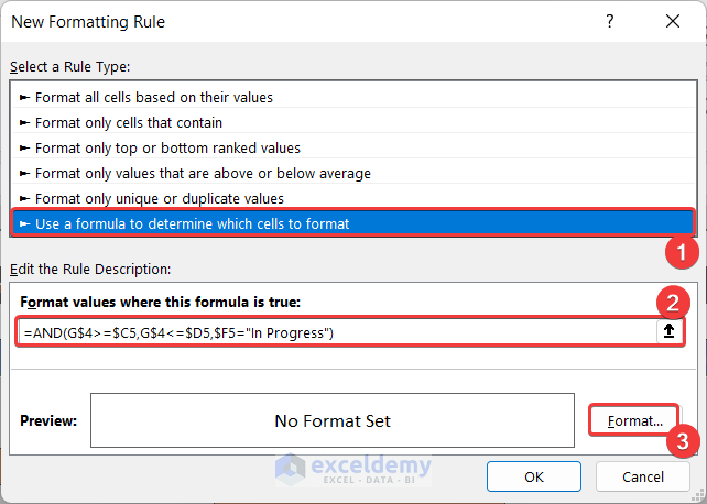
- Choose a color for this category. We chose Green, Accent 6, Lighter 40%.
- The In Progress projects shows the selected color.
- Create another formatting rule for the Pending
- Enter the following formula in the New Formatting Rule dialog box,
=AND(G$4>=$C5,G$4<=$D5,$F5="Pending")
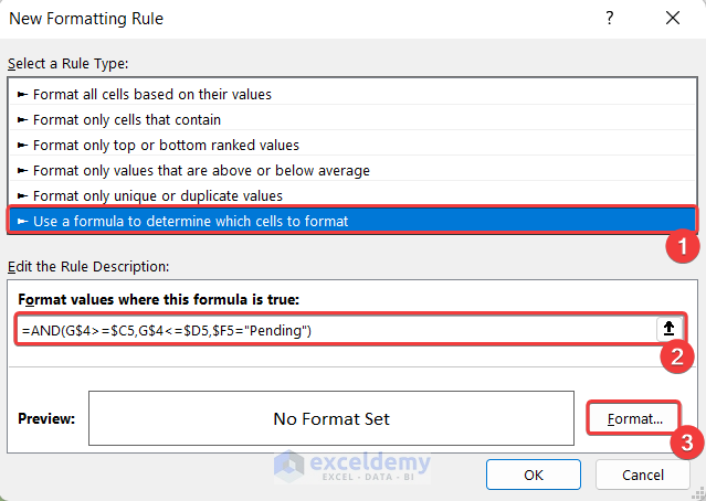
- Choose another color from the Fill tab of the Format Cells dialog box. We chose Red for this category.
- Close all the dialog boxes and you will get the complete Gantt chart.
Download Practice Workbook
Related Articles
- How to Use Excel Gantt Chart
- How to Add Milestones to Gantt Chart in Excel
- How to Show Dependencies in Excel Gantt Chart
<< Go Back to Gantt Chart Excel | Excel Charts | Learn Excel
Get FREE Advanced Excel Exercises with Solutions!
