What Is a Gantt Chart?
The Gantt chart was popularized by Henry Gantt. It is a type of bar chart that illustrates or tracks a project schedule. It lists activities or tasks on the left of the bar chart a time frame for them. Here is how a Gantt Chart usually looks like:
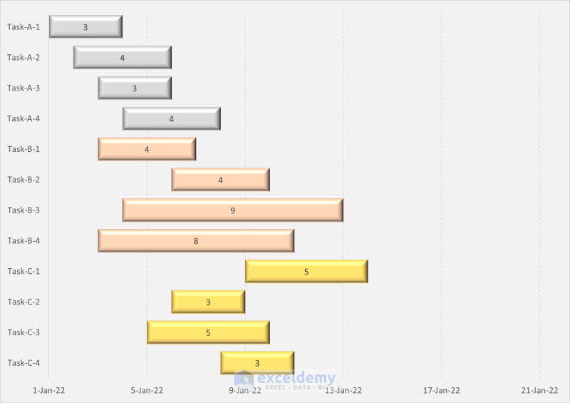
A Gantt chart can be used to determine:
- Total different activities
- When each of them starts or ends
- How long they last
- If there are any overlaps or gaps in between them.
How to Create Excel Gantt Chart with Multiple Start and End Dates: Step-by-Step Procedure
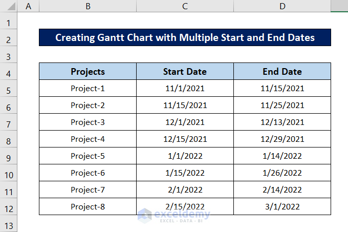
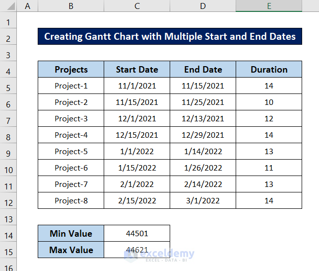
For example, let’s take a dataset where there are multiple projects with multiple start and end dates.
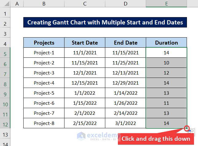
Step 1 – Calculate Duration of Each Project
- Select cell E5 and copy the following formula:
=D5-C5
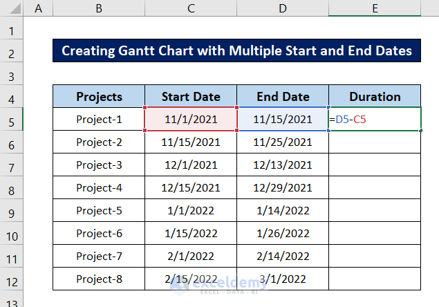
- After pressing Enter, you will have the duration of the first project.
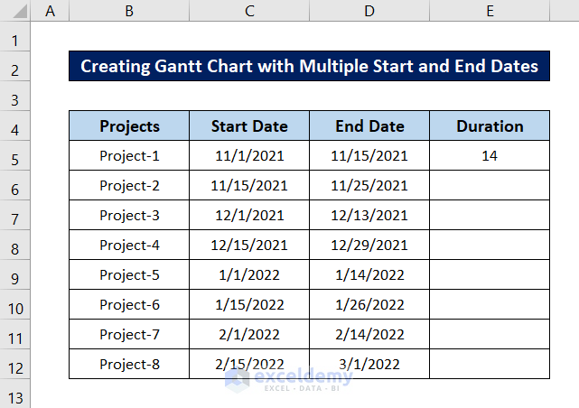
- Select the cell again and click and drag the fill handle icon down to replicate the formula for the rest of the cells.
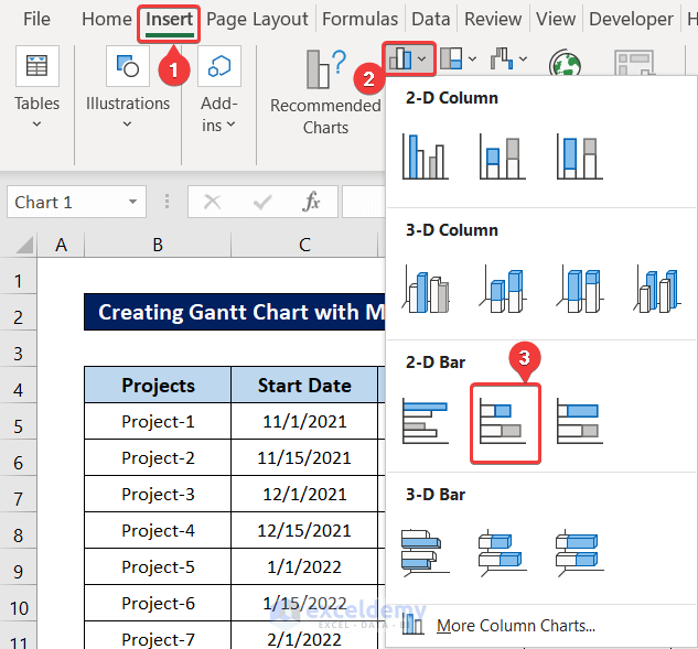
Step 2 – Create Stacked Bar Chart
- Select a cell and go to the Insert tab on your ribbon.
- Pick the Insert Column or Bar Chart option from the Charts group.
- Choose Stacked Bar from the 2-D Bar section of the drop-down menu.
Read More: How to Show Dependencies in Excel Gantt Chart
Step 3 – Select Data for Stacked Bar Chart
Let’s reconfigure the blank stacked bar chart made from the previous step:
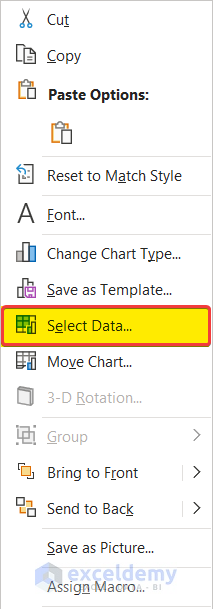
- Right-click on the chart area.
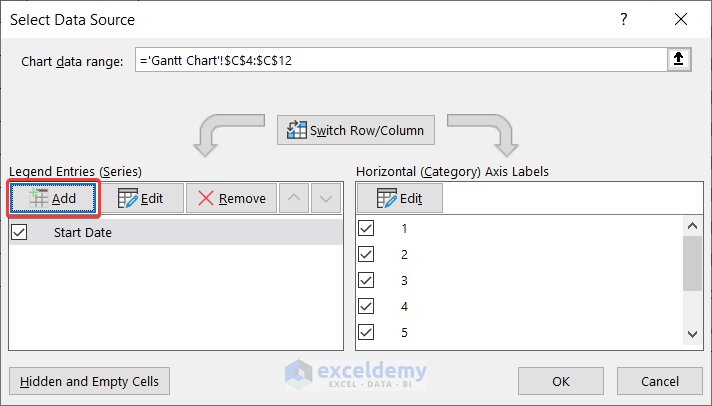
- Choose Select Data from the context menu.
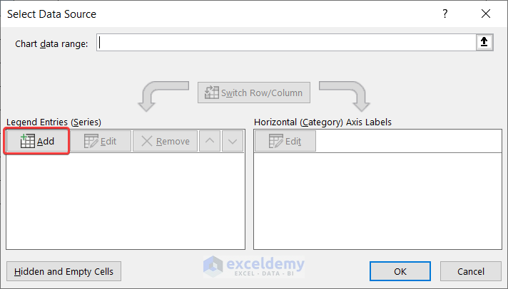
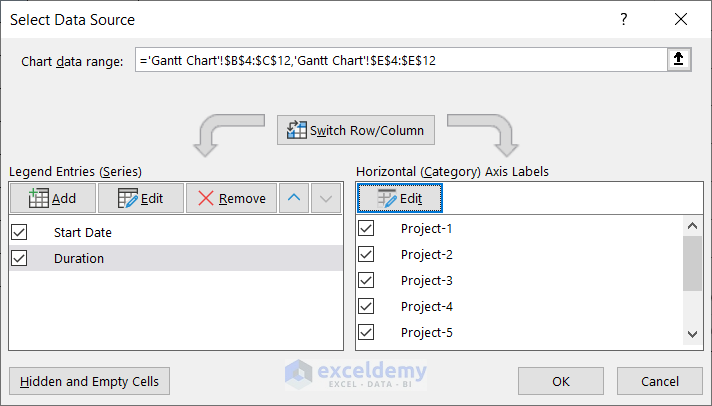
- The Select Data Source box will appear. Click Add under Legend Entries first.
- In the Edit Series box, select cell C4 for Series name and select the range C5:C12 for Series values.
- Click on OK.

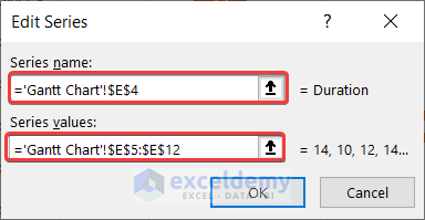
- Click on Add again under Legen Entries in the Select Data Source box.
- Select cell E4 as the Series name and the range E5:E12 as the Series values.
- Click on OK.
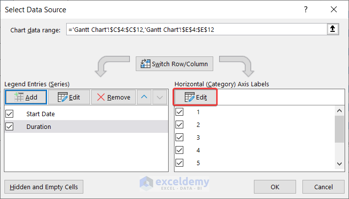
- Click on Edit under Horizontal Axis Labels in the Select Data Source box.
- Select the range B5:B12 as the Axis label range in the Axis Labels box and click on OK.
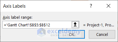
- Press OK in the Select Data Source box.
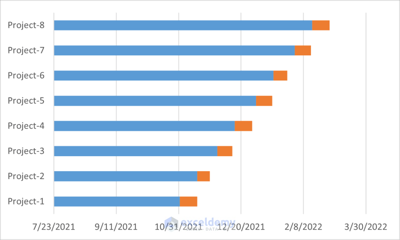
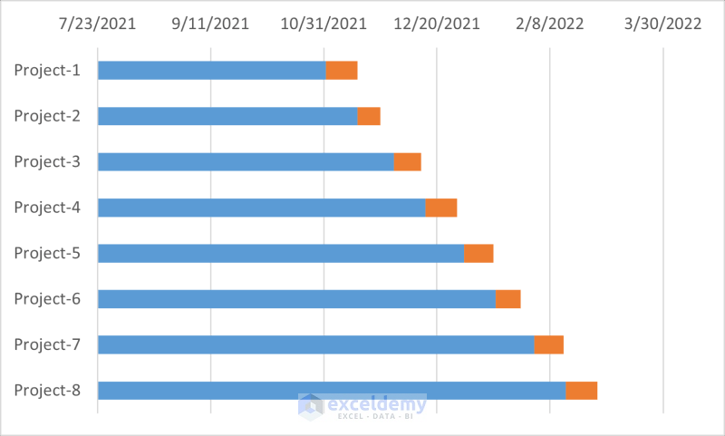
- The graph will look like this now.
Read More: How to Add Milestones to Gantt Chart in Excel
Step 4 – Reverse Order of Categories
In the graph created at the end of the previous step, the project orders are in the opposite order. Let’s reverse them.
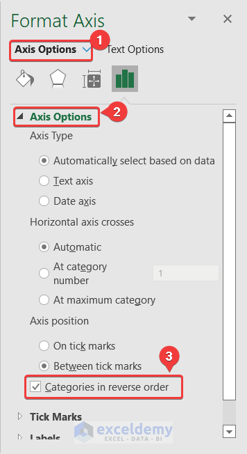
- Double-click on the axis. This will open up the Format Axis window on the right of the spreadsheet.
- Select the Axis Options section in the Axis Options tab.
- Check the Categories in reverse order option.
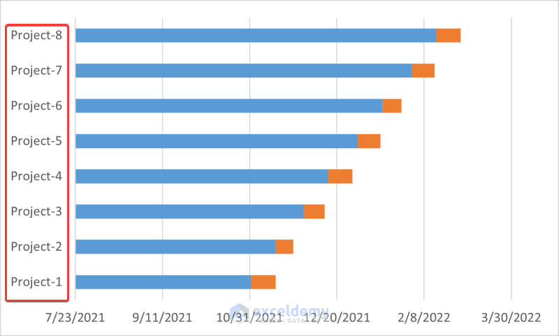
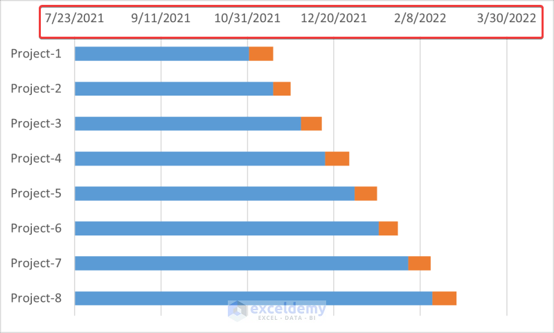
- The graph will look something like this.
Step 5 – Readjust Horizontal Axis Label Position
After rearranging the project lists in the previous step, the horizontal axis labels will move up, and we need them down.
- Double-click on the axis label.
- The Format Axis window will pop up on the right of the spreadsheet.
- Go to the Axis Options tab and under the Labels section, change the Label Position to High.
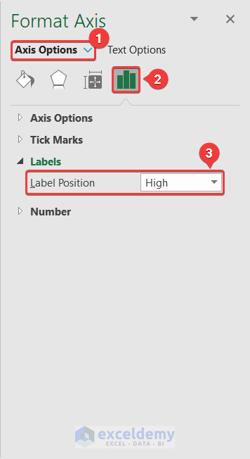
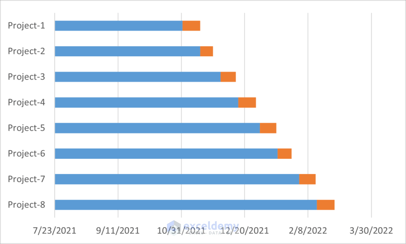
- The horizontal axis label will automatically shift down to its original position again.
Step 6 – Remove Fills and Borders of Start Dates
A standard Gantt chart only represents the duration and starting point of a task. But the chart we have created has both the starting date as well as the durations plotted from a base starting date of 7/23/2021. We need to remove these blue bars.
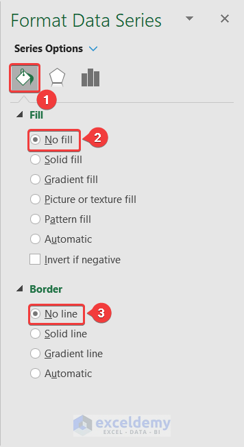
- Double-click on any of the blue bars in the chart.
- The Format Data Series window will open up on the right of the spreadsheet. Select the Fill & Line tab here.
- Select No fill for both the Fill and Border sections.
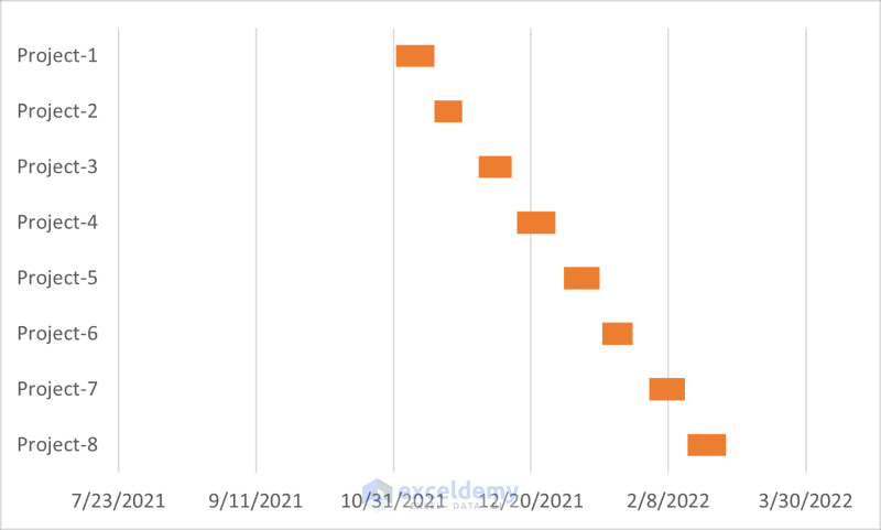
Now the chart will look closer to a Gantt chart.
Step 7 – Change Maximum and Minimum Values of Horizontal Axis
The chart seems to start and end at a random date. We need to modify it more to look more like an ideal Gantt chart that starts and ends with the horizontal axis.
- To determine the maximum and the minimum value of the axis find when the earliest project starts and the latest project ending date. These dates are located in cells C5 and D12 in our dataset.
- Copy and paste the values to another cell or use a MIN and MAX formula to extract them dynamically. We have pasted them in cells C14 and C15 for demonstration.
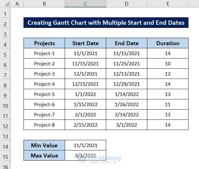
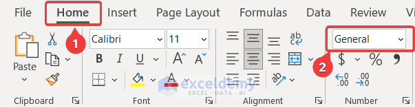
- Select the cells and change the cell format to General. You can find it in the Number group of the Home tab.
- The values will look something like this.
- To change the chart label values to these, double-click on the horizontal axis label.
- The Format Axis window will open up within the Excel spreadsheet. Go to the Axis Options tab in it.
- Put the values obtained in the value boxes under the Axis Options section.
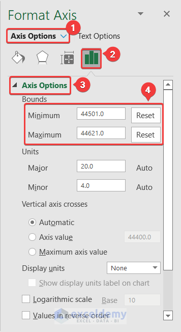
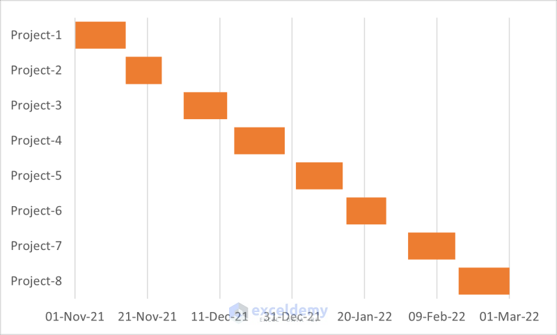
- The chart will look like this.
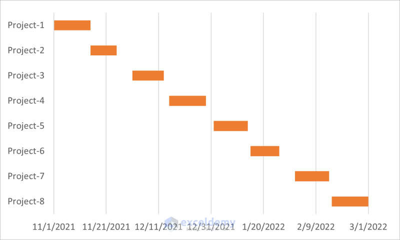
Step 8 – Format Gantt Chart
- Double-click on the horizontal axis label.
- The Format Axis window will open up again. Go to the Axis Options tab in it.
- Under the Number section, you can find the Format Code. Type in any format you like. We have selected dd-mmm-yy as the date format.
- Click on Add.
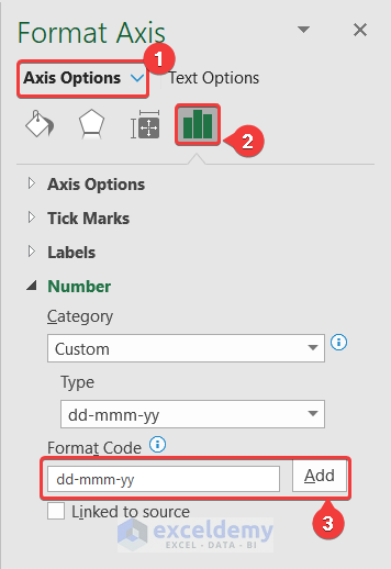
The graph label will change now.

- You can also make the bars thicker by double-clicking them and changing the Gap Width from the Series Options tab to a lower value.
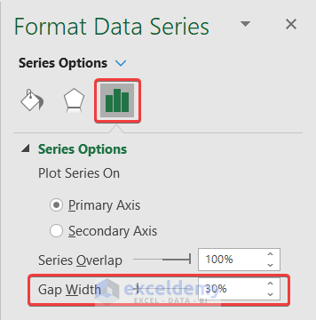
Here’s an example of changing the width.
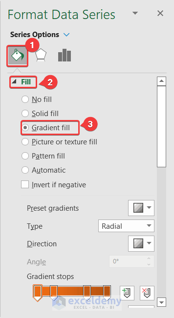
- You can change the fill color/style from the same window. Go to the Fill & Line tab and select your style under the Fill section. We have selected gradient fill as our style.
- You can also add labels by selecting the chart and clicking on the Chart Elements icon that appears on the right, then selecting Data Labels.
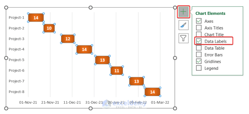
The chart will finally look like this.

Read More: How to Use Excel Gantt Chart
Download Practice Workbook
You can download the workbook with the dataset and the Gantt chart of the demonstration from the link below.
Related Article
- How to Make a Gantt Chart in Excel
- How to Create Gantt Chart for Multiple Projects in Excel
- Excel Gantt Chart with Conditional Formatting
<< Go Back to Gantt Chart Excel | Excel Charts | Learn Excel
Get FREE Advanced Excel Exercises with Solutions!

In Step 6 (Step 6: Remove Fills and Borders of Start Dates), where did the date of 7/23/2021 come from?
Greetings ALAN,
I appreciate you asking this question. Excel will automatically generate this date in the intermediate stage when you are trying to create a gannt chart. During the Final stage, you will notice that project-1’s starting date has been corrected.
Hi, this was a clear guideline, thank you. I have an additional question. I want to have different bars for 1 project behind each other. Is that possible?
For example
project start end duration start end duration
1 1.1. 31.1. 31 1.6. 30.6. 30
2 1.1. 31.3. 89
Hi Elly,
For your data, plotting a stacked bar chart would not be possible. Excel needs a dataset of the following sort to plot a stacked bar chart.
1st Week 2nd Week 3rd Week 4th Week
1st Task 44 41 61 58
2nd Task 38 52 53 64
3rd Task 42 48 50 56
4th Task 37 59 44 46
Even in that case, creating a Gantt chart would not be appropriate, as one bar will start where the previous one ended. This will ultimately result in the same bar plot. But if you have a gap between each work period, you can put them in between these values and follow the steps of the article.
Thanx very Much,
Your information has helped me to gain Favor from My Boss Since i had No Idea About this chart and it was badly wanted for Information reporting!
Dear Ronald,
You are most welcome.
Regards
ExcelDemy