Complex numbers are expressed as a+ib, where “a” is a real part of the complex number and “b” is an imaginary part of the complex number. For instance, the complex number 4+3i is made up of the real number 4 (Re) and the imaginary number 3i (Im). Often, you may have complex number coefficients, or even complex numbers in polar format. In such a situation, how can you format the complex numbers in the a+ib format? Well, this article focuses on 4 suitable ways of how to format complex numbers in Excel.
Format Complex Numbers in Excel: 4 Methods
In this section, we have covered 4 methods for 3 different datasets. The first two methods deal with the formatting of complex numbers when the dataset contains coefficients. You can use the third method if you find the complex number in cartesian form. The last shows the use of VBA code.
Here, we have used the Microsoft Excel 365 version; you may use any other version according to your convenience.
1. Using COMPLEX Function
The COMPLEX function is the most efficient and easy way that we have found to format your complex number. Basically, the COMPLEX function creates a complex number of the form x + iy using real and imaginary coefficients. Now the question is, “How will you do that?” Well, all you have to do is call the COMPLEX function before putting its arguments in a specific cell.
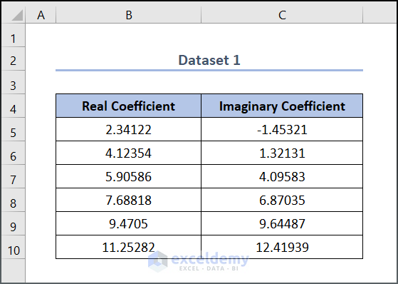
Let’s assume we have a dataset, namely “Dataset 1”. As a complex number consists of two parts, we have created two columns named Real Coefficient and Imaginary Coefficient. However, you can use any data set that is suitable for you.
📌 Steps:
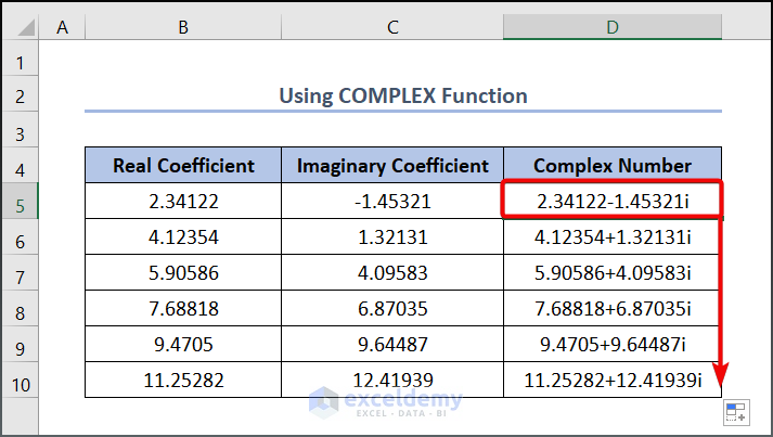
- Write the following formula in cell D5.
=COMPLEX(B5,C5)- Press the Enter button afterwards.

- Drag the Fill Handle tool to get the other values.
Read More: How to Display Long Numbers in Excel
2. Applying COMPLEX and ROUND Functions Simultaneously
Now what if you want to avoid seeing those extra decimal digits in your output list? Well, in this case, you can incorporate the ROUND function into your formula editor along with the COMPLEX function to make your output short.
📌 Steps:
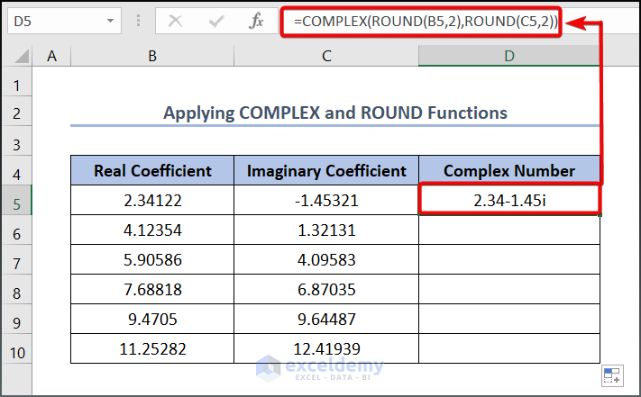
- To begin with this method, enter the following formula in cell D5.
=COMPLEX(ROUND(B5,2),ROUND(C5,2))Here, B5 and C5 cells refer to Real Coefficient and Imaginary Coefficient respectively.
In the above formula, the ROUND(B5,2) syntax returns the real coefficients in the B5 cell with 2 digits. And the output is 2.34.
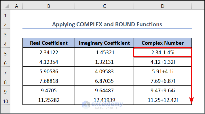
- To get the other value, drag the Fill Handle tool from D5 to D10.
Read More: How to Change Decimals to Percentages in Excel
3. Employing SIN and COS Functions
If your input values are in polar form but you want to format them in cartesian form, the method we’ll go over is for you. We will employ the SIN and COS functions in our formula editor to accomplish the desired output. But first, look at the dataset we have attached below.
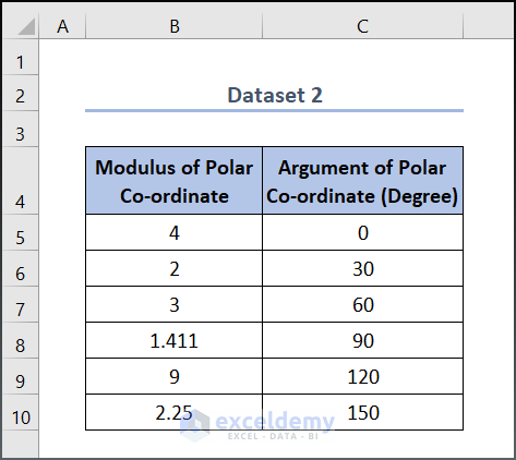
As the polar form of a complex number is comprised of two values, we have created two columns (for modulus and argument).
📌 Steps:
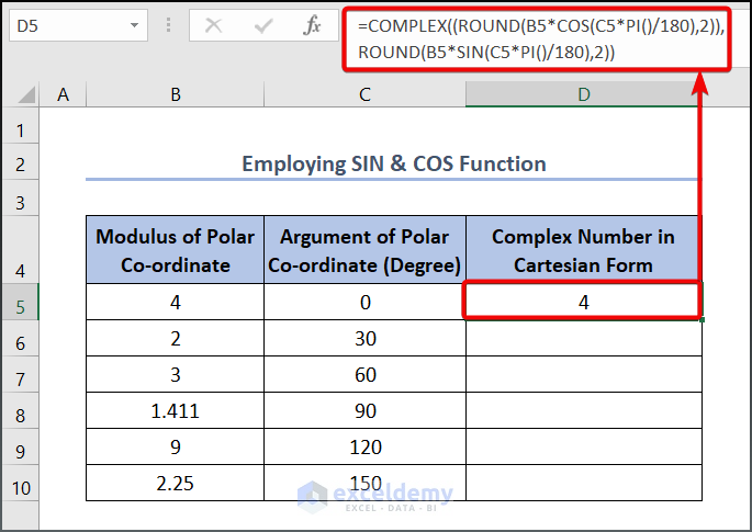
- Write the following formula in cell D5.
=COMPLEX((ROUND(B5*COS(C5*PI()/180),2)),ROUND(B5*SIN(C5*PI()/180),2))Here, B5 & C5 cells refer to Modulus of Polar Co-ordinate and Argument of Polar Co-ordinate respectively.
- Subsequently, press the Enter button.
Formula Breakdown
- COS(C5*PI()/180) → returns the cosine value of the number of the C4
- Output →1
- (ROUND(B5*COS(C5*PI()/180),2) → returns the multiplication of B5 cell and cosine value of C4 cell with 2 digits.
- Output → 1
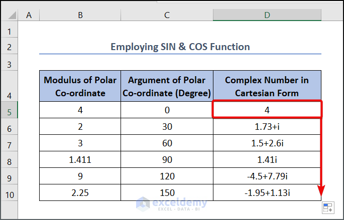
- Drag the Fill Handle tool to get the other values.
4. Incorporating VBA Code
Now, if you wish to accomplish your task by incorporating VBA code, then follow the method that we are going to describe below. Here we will calculate as well as format a square root of a negative number using an Excel spreadsheet.
📌 Steps:
- Press Alt + F11 to open your Microsoft Visual Basic.
- Then press Insert > Module to open a blank module.
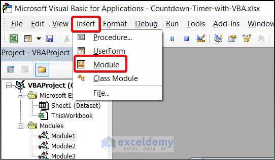
- Now, write the following VBA code in your
Function ComplexFormatting(A As Variant, temp As String) As String
With Application.WorksheetFunction
ComplexFormatting = Format(.ImReal(A), temp) & Format(.Imaginary(A), temp) & "i"
End With
End Function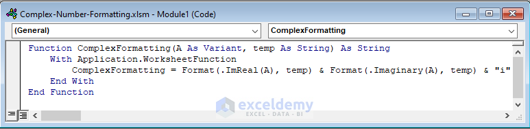
Now, we will explain how the given VBA code works.
⚡ Code Breakdown:
The code is divided into 2 steps.
- In the first portion, there are two variables named “a” as Variant and “temp” as String to keep the cell values.
- In the second portion, WorksheetFunction has been incorporated to collect the property of the application object to return the WorksheetFunction The cell values will be formatted once it is retrieved from their corresponding cells.
- Close your VBA window.
- Right now, a function named ComplexFormatting is created!
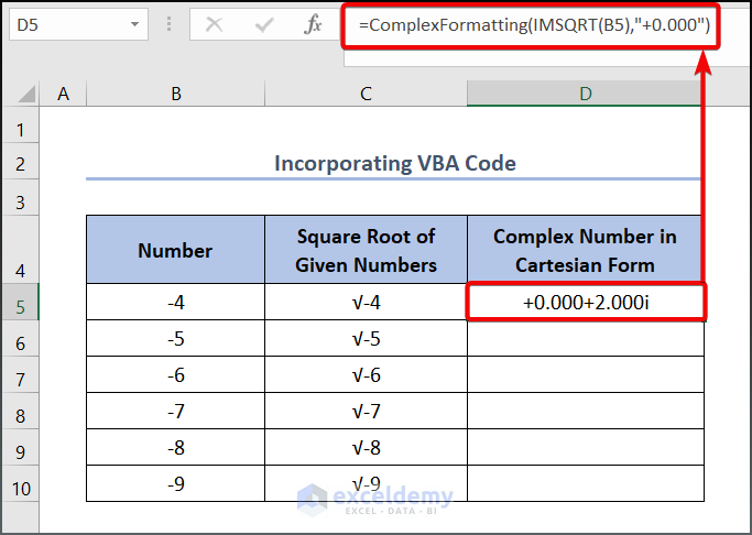
- Next, write the following formula in D5 cell.
=ComplexFormatting(IMSQRT(B5),"+0.000")- Press the Enter button, and see the output given below.
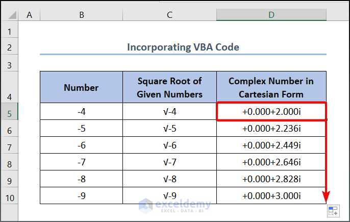
- Drag the Fill Handle tool to get the other values.
Practice Section
We have provided a Practice section on the right side of each sheet so you can practice yourself. Please make sure to do it yourself.
Download Practice Workbook
You can download and practice the dataset that we have used to prepare this article.
Conclusion
In this article, we have discussed how to format complex numbers in Excel. As you have already understood, there are plenty of ways to do this task. So before going through a specific method, ensure the method you choose aligns with your work. Further, if you have any queries, feel free to comment below and we will get back to you soon.
Related Articles
- How to Change Comma to Dot in Excel
- How to Change International Number Format in Excel
- How to Enter 16 Digit Number in Excel
- How to Enter 20 Digit Number in Excel
<< Go Back to Number Format | Learn Excel
Get FREE Advanced Excel Exercises with Solutions!
