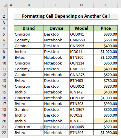
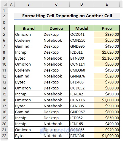
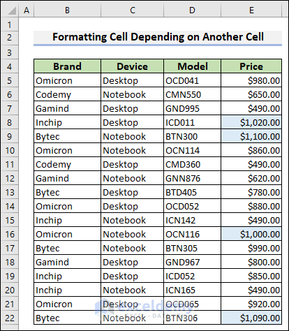
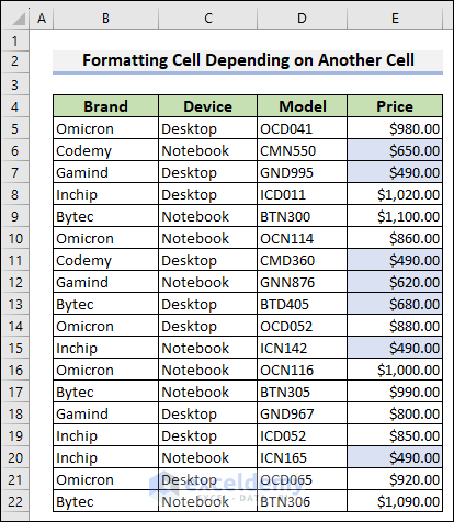
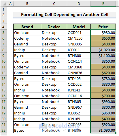
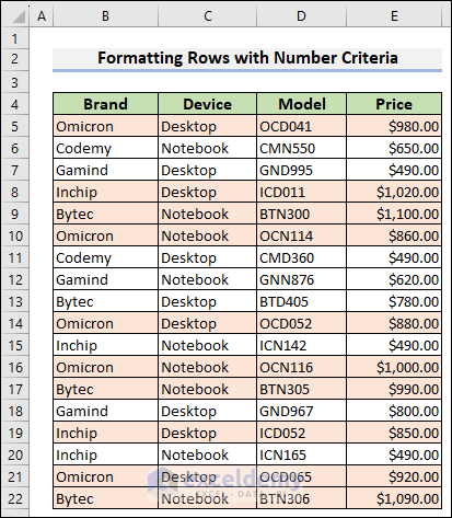
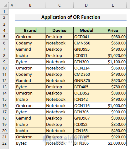
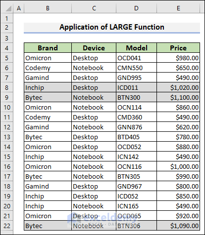
The following dataset represents the Devices of several Brands, Models, and Prices of those Devices. We will use it to demonstrate how to format cells based on its contents.
How to Open a New Formatting Rule Window from Conditional Formatting Feature in Excel
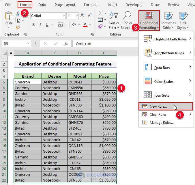
- Select the range B5:E22.
- Go to the Home tab and the Styles group.
- Choose Conditional Formatting and select New Rule.
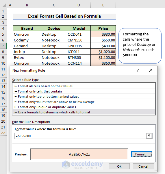
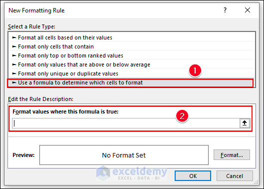
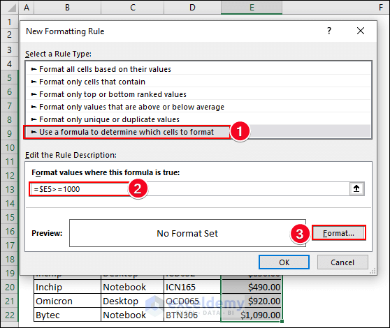
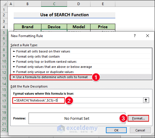
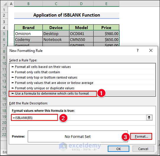
- A window named New Formatting Rule will pop up. Choose the Use a formula to determine which cells to format option for select a Rule Type.
- In the field Format values where this formula is true, use a formula to format cells as you want.
Notes:
This procedure will be used to pop up the New Formatting Rule window in each of the examples below.
Method 1 – Using an Excel Formula to Format a Cell Depending on Another Cell
Let’s format the Sales cells based on various requirements.
Case 1 – Equal To $490.00
- Select the range E5:E22.
- Open the New Formatting Rule window.
- In the Format values where this formula is true box, use the following formula:
=$E5=490- Pess Format.
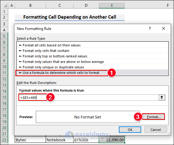
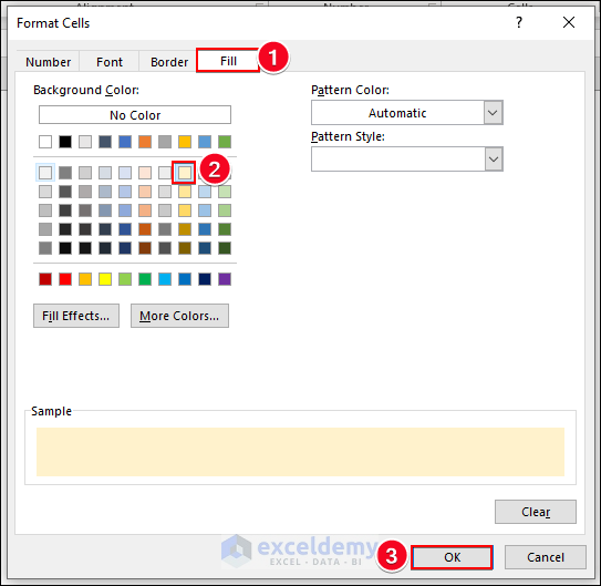
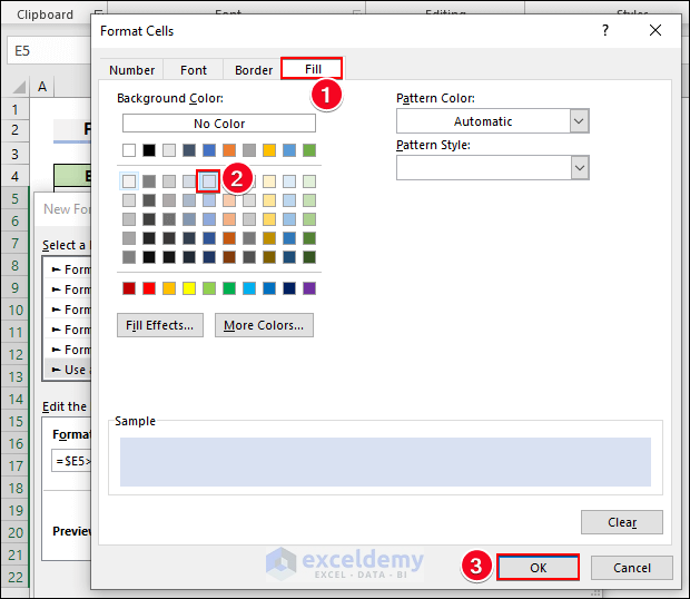
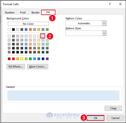
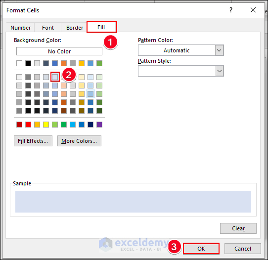
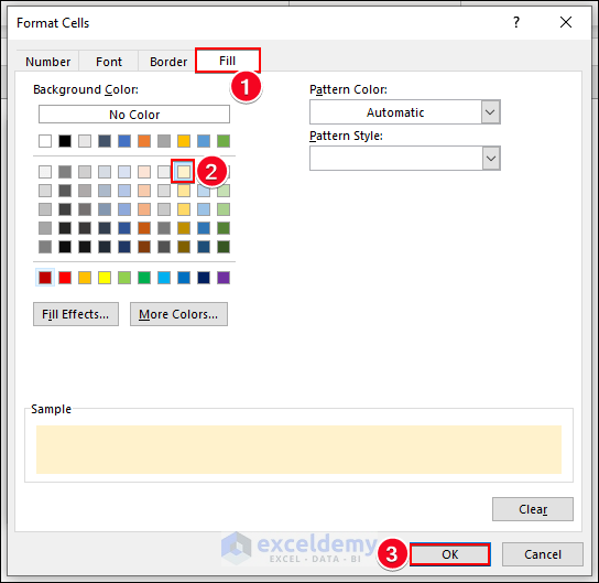
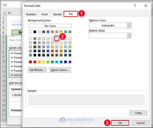
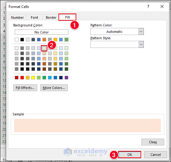
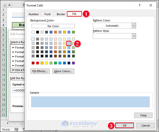
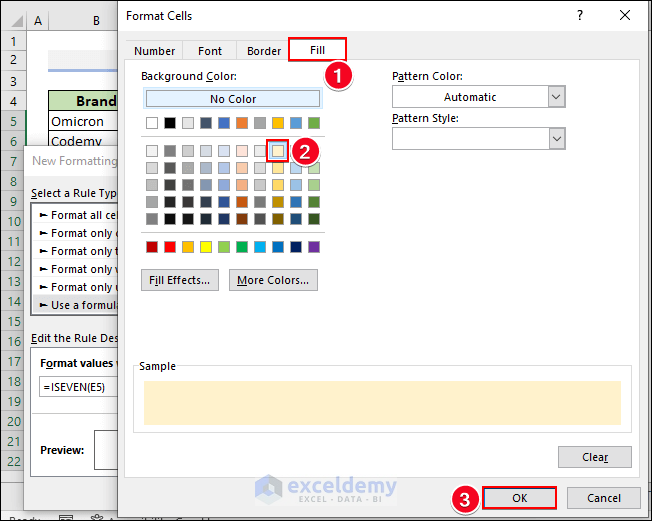
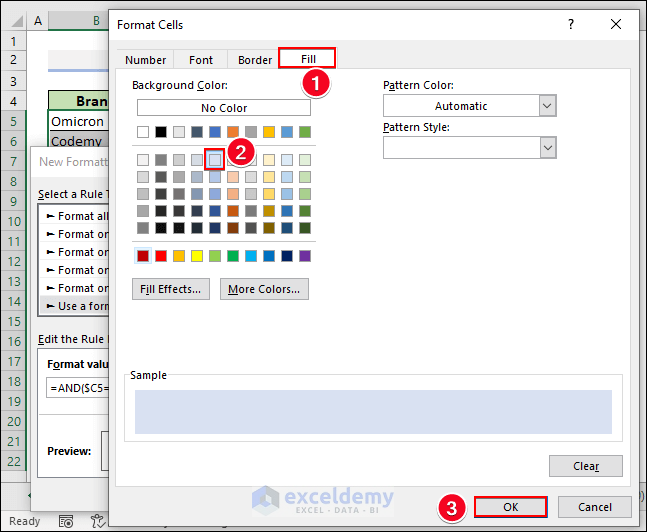
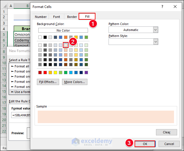
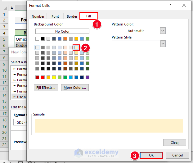
- The Format Cells dialog box will pop out. Under the Fill tab, select a color and press OK.
- You’ll see the highlighted cells which are equal to E5.
Case 2 – Not Equal To $490.00
- Type the following formula in the New Rule and press Format:
=$D5<>490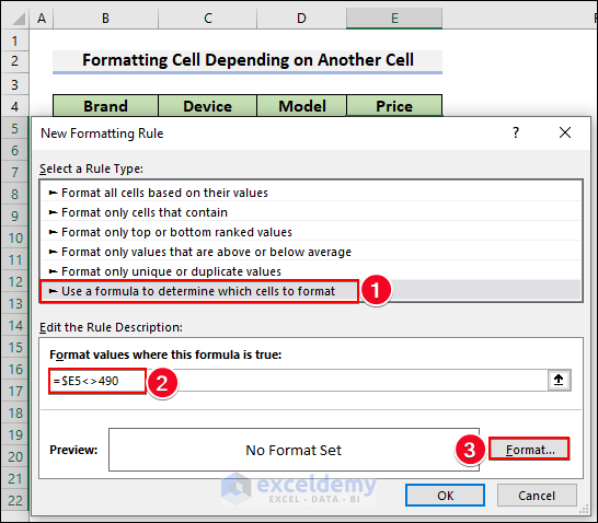
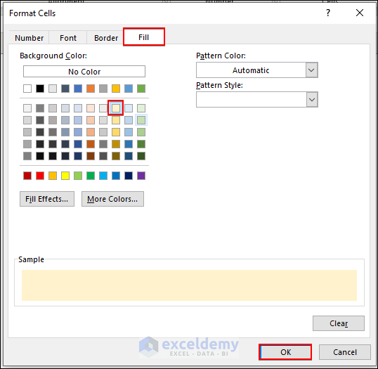
- The Format Cells dialog box will pop out. Under the Fill tab, select a color.
- Press OK.
- You’ll see the desired changes.
Case 3 – Greater Than $1,000.00
- Use the following formula and press Format.
=$D5>1000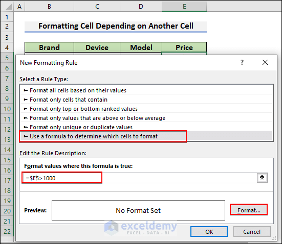
- Select any color from the Fill tab and hit OK.
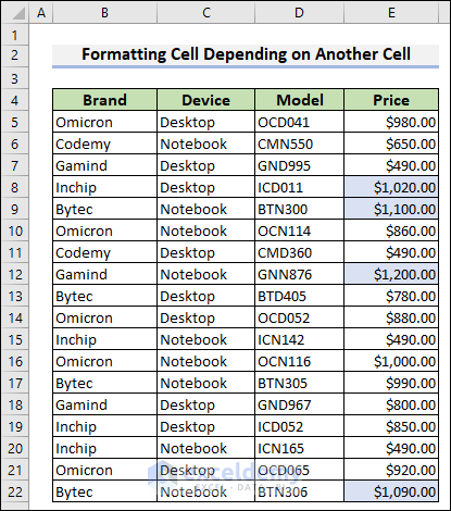
- You’ll see the highlighted cells whose values are greater than $1,000.00.
Case 4 – Greater Than or Equal To $1,000.00
- Use the following formula:
=$D5>=1000- Press Format.
- Format the color as you want.
- You’ll be able to highlight cells whose values are greater than or equal to $1,000.00.
Case 5 – Less Than $700.00
- Insert the following formula and select Format.
=$D5<700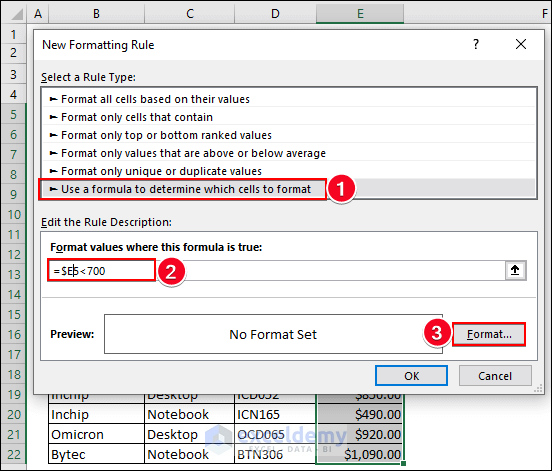
- Choose your formatting and press OK.
- You’ll see the highlighted cells whose values are less than $700.00.
Case 6 – Less Than or Equal To $700.00
- Use the following formula and choose Format.
=$D5<=700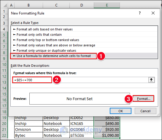
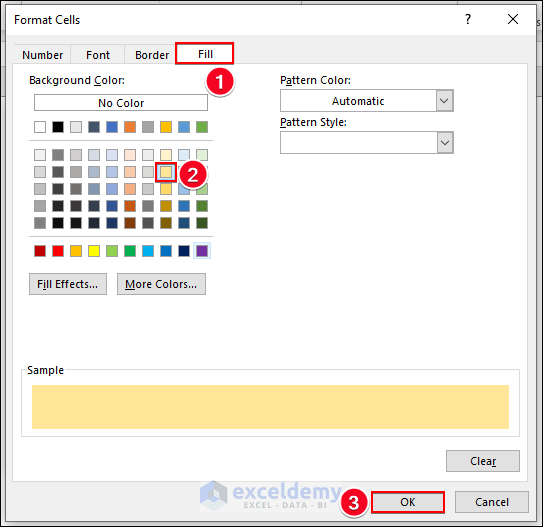
- Choose your formatting and press OK.
- You’ll see your desired highlighted cells.
Case 7 – Between $600.00 and $1,000.00
- Use the following formula:
=AND($E5>600, $E5<1000)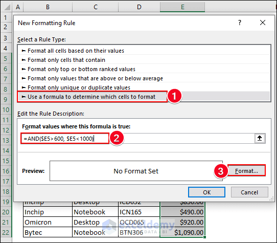
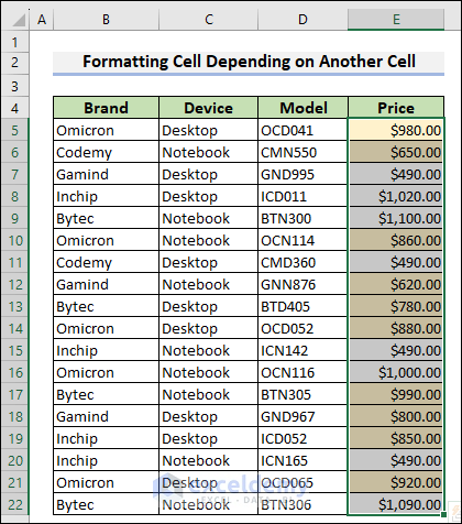
- Format the cells as you want them and press OK.
- It’ll return the formatted cells.
Read More: How to Do Conditional Formatting Based on Another Cell in Excel
Method 2 – Applying an Excel Formula to Format Rows with Text Criteria
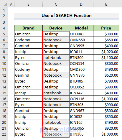
In the below dataset, we’ll look for a product Notebook and format the rows where the product is present.
Case 1 – Using the SEARCH Function: Case-Insensitive
- Select cell range C5 to C22.
- Make a New Conditional Formatting rule and insert the following formula in Format values where this formula is true.
=SEARCH(“Notebook”,$C5)>0- Click on Format.
- Choose any color from the Fill tab and select OK.
- The SEARCH function returns the formatted cells with the case-insensitive issue.
Read More: How to Apply Conditional Formatting to Each Row Individually
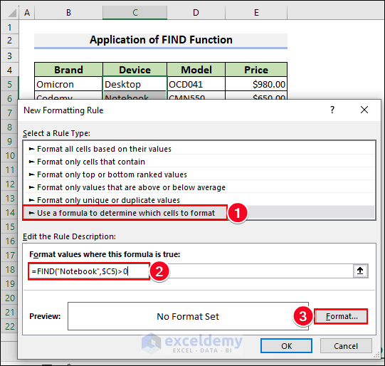
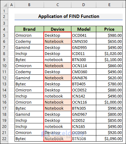
Case 2 – Applying the FIND Function: Case Sensitive
- Use the following formula in the Format values where this formula is true box.
=FIND(“Notebook”,$C5)>0- Select Format.
- Select a formatting color and press OK.
- You’ll see the highlighted cells containing only “Notebook” values, not “notebook”.
Read More: How to Change Row Color Based on Text Value in Cell in Excel
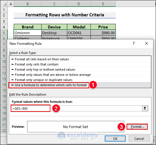
Method 3 – Formatting Rows with Number Criteria Based on Formula
We’ll format the rows where the price of a Desktop or Notebook exceeds $800.00.
- Use the following formula for a New Conditional Formatting Rule:
=$E5>800- Press Format.
- Choose a fill color and press OK.
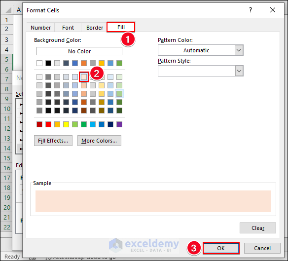
- It’ll return the desired rows in the specified color.
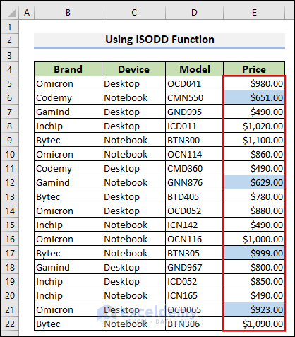
Method 4 – Formatting Odd Numbered Cells in Excel Based on Formula
- Use the following formula in the Conditional Formatting rule box:
=ISODD(E5)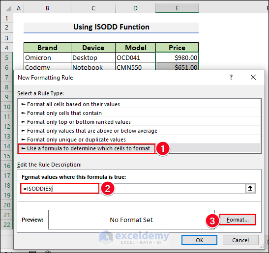
- Apply formatting as you want and click on OK.
- You’ll see the odd numbers in the selected color.
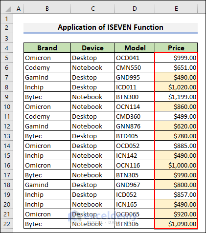
Method 5 – Using Excel Formula to Format Even Numbered Cells
- Use the following formula in the Conditional Formatting Rule box:
=ISEVEN(E5)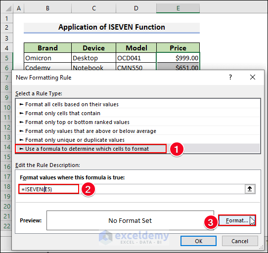
- Apply formatting and press OK.
- You’ll see the even numbers in the selected color.
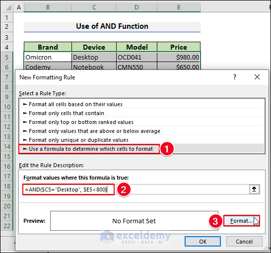
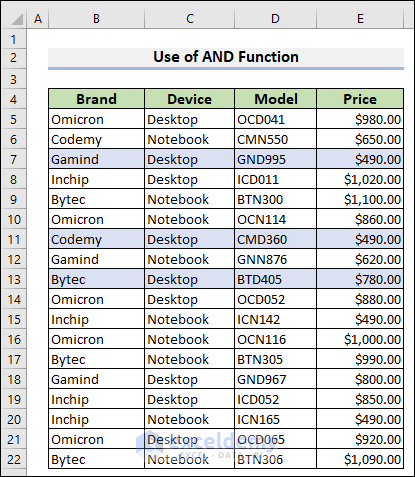
Method 6 – Applying Excel Formula with the AND Function to Format Cells
We’ll highlight the rows which contain the product Desktop with the Price below $800.
- Use the following Conditional Formatting formula:
=AND($C5="Desktop", $E5<800)- Select Format.
- Choose a fill color and press OK.
- It’ll return the formatted rows.
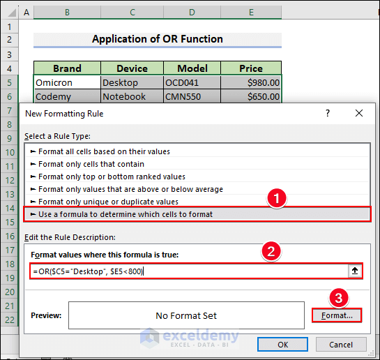
Metho 7 – Formatting Cells with the OR Function in Excel
- Insert the following formula into the Conditional Formatting rule box:
=OR($C5="Desktop", $E5<800)- Press Format.
- Choose a fill color and press OK.
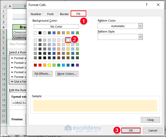
- The OR function will return the formatted rows.
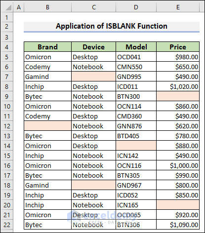
Method 8 – Applying the ISBLANK Function to Format Blank Cells
- Use the following formula inside the Conditional Formatting Rule box:
=ISBLANK(B5)- Press Format.
- Choose a fill color and press OK.
- The ISBLANK function will highlight the blank cells.
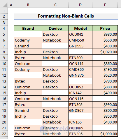
Method 9 – Formatting Non-Blank Cells Based on Excel Formula
- Use the following formula into the Conditional Formatting rule box:
=NOT(ISBLANK(B5))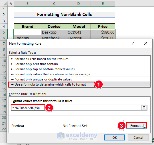
- Select any color to fill the cells and press OK.
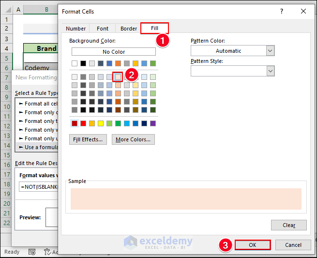
- You will format the non-blank cells.
Method 10 – Formatting Duplicate Cells Based on Formula
Case 1 – Formatting Duplicate Cells Including First Occurrences
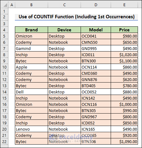
Let’s check for repeated brand names (column B):
- Use the following formula in the Conditional Formatting rule box:
=COUNTIF($B$5:$B$22,$B5)>1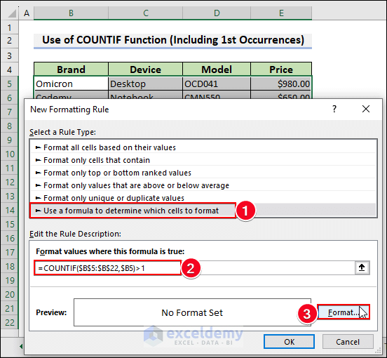
- Pick your preferred formatting and press OK.
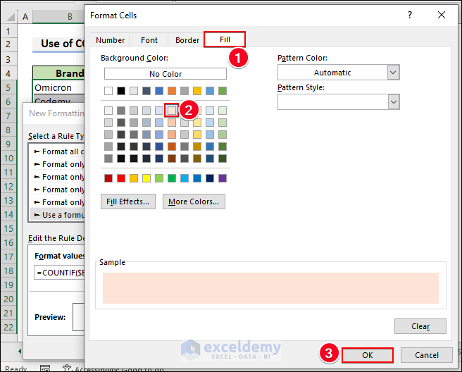
- This will return the duplicate information across rows including the first occurrences.
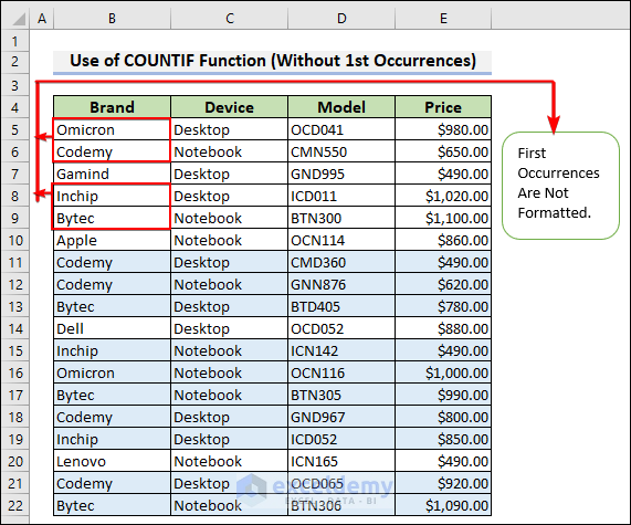
Case 2 – Formatting Duplicate Cells Without First Occurrences
- Use the following formula in the Conditional Formatting box:
=COUNTIF($B$5:$B5,$B5)>1- Now press Format.
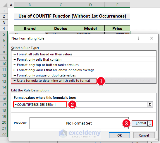
- Go to Format and pick a fill color, then press OK.
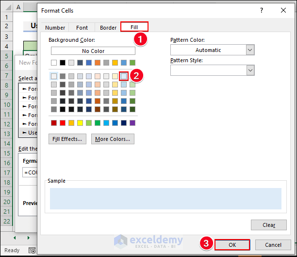
- This will return the highlighted rows without the first occurrences.
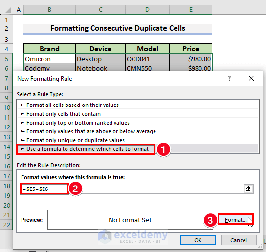
Case 3 Formatting Consecutive Duplicate Cells in Excel
Let’s repeat the duplicate check for brand names but highlight only consecutive duplicates:
- Use the following formula in the Conditional Formatting rule box:
=$B5=$B6- Press Format.
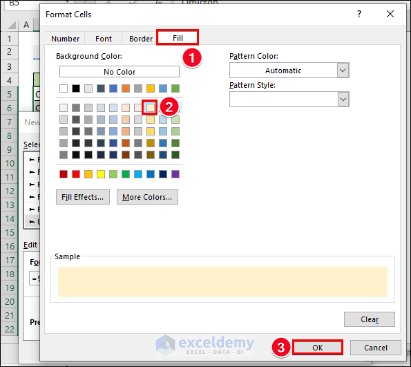
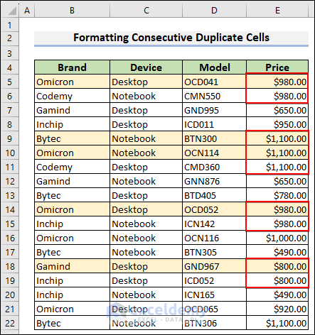
- Choose your formatting and press OK.
- Apply and you’ll get consecutive duplicate cells.
Method 11 – Using the Excel AVERAGE Function to Format Cells
Case 1 Formatting Cells Greater Than Average Value
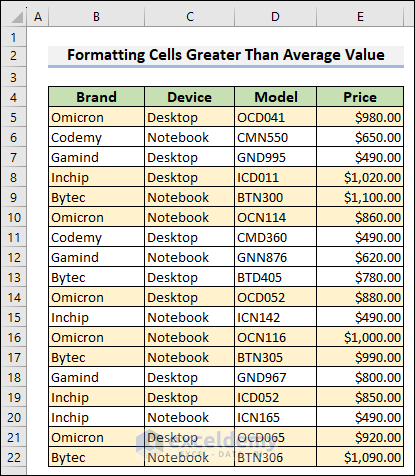
We will format the rows in which the price of the products is greater than the average.
- Insert the following formula into the Conditional Formatting rule box:
=$E5>AVERAGE($E$5:$E$22)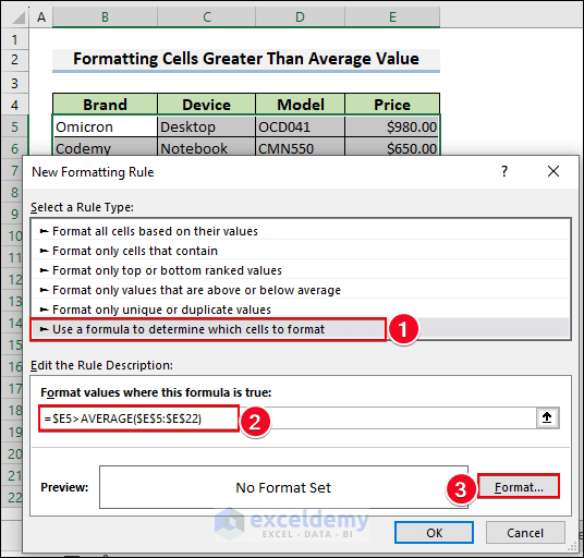
- Choose your formatting in the Format box.
- You’ll get the highlights.
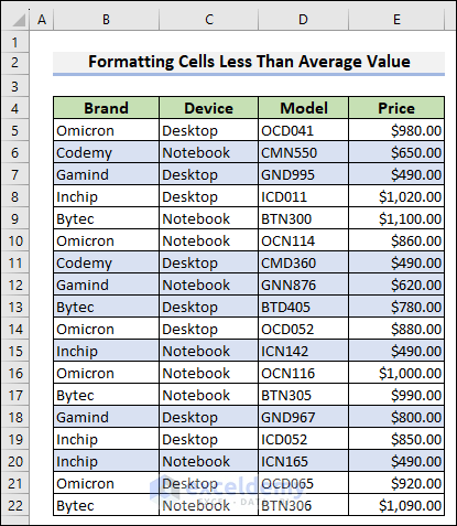
Case 2 – Formatting Cells with Lower Than the Average Value
- Insert the following formula into the Conditional Formatting rule box:
=$E5<AVERAGE($E$5:$E$22)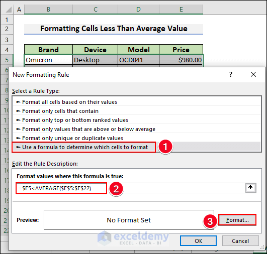
- Choose your preferred formatting in the Format option.
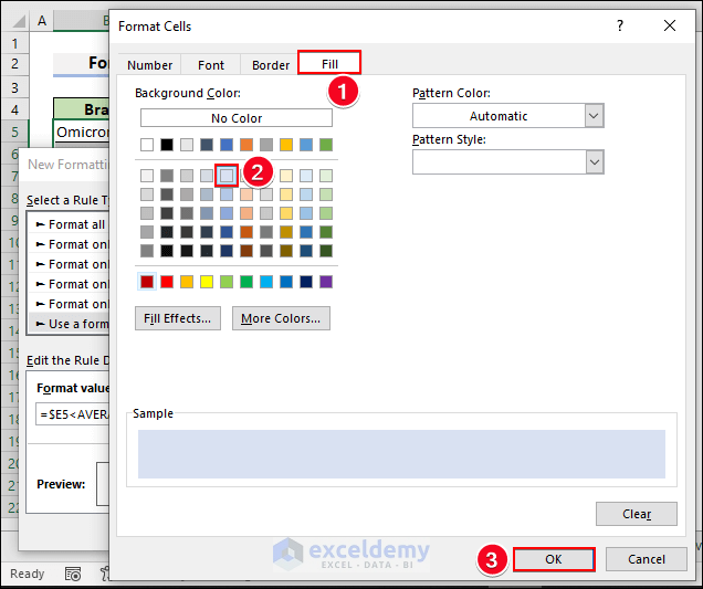
- You’ll get the desired output.
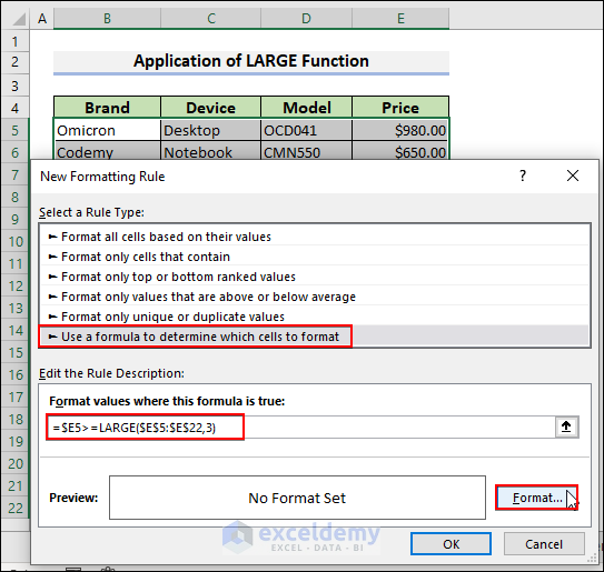
Method 12 – Formatting Cells with Top 3 Values Based on Formula
We’ll use a function to format the rows with 3 top prices of the products.
- Insert the following function into the Conditional Formatting rule box:
=$E5>=LARGE($E$5:$E$22,3)- Press Format.
- Choose a fill color and press OK.
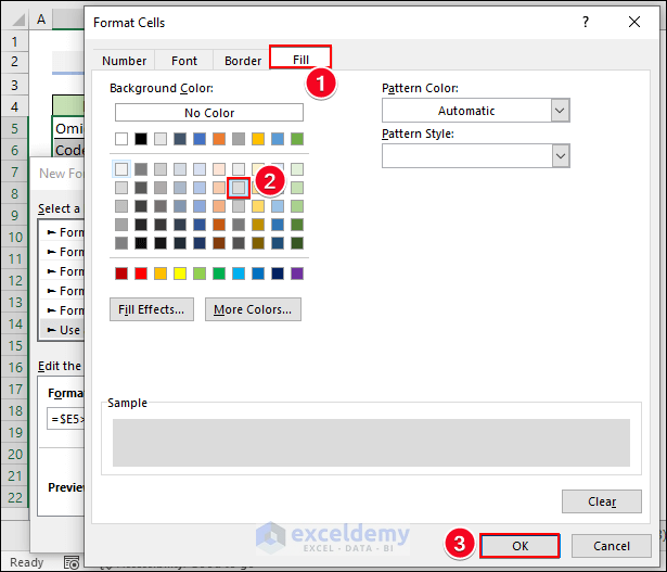
- This will return the expected output.
Method 13 – Formatting Entire Rows with Excel Formula When Any Cell Is Blank
- Use the following formula in the Conditional Formatting rule box and press Format:
=COUNTBLANK($B5:$E5)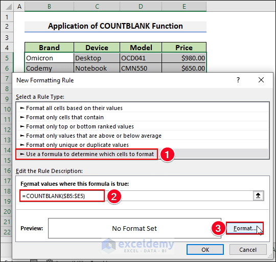
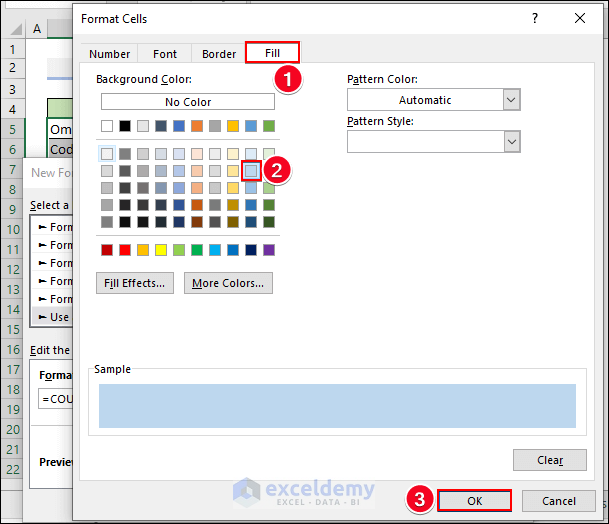
- Select any color to fill the cells and press OK.
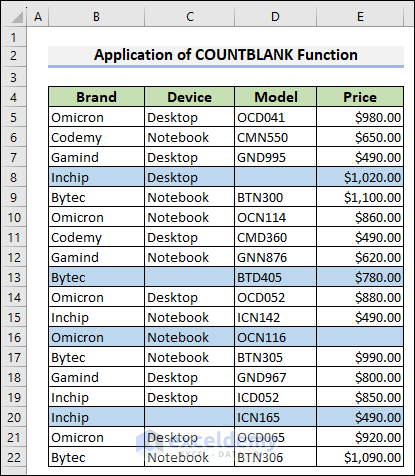
- This’ll return the dataset highlighting the rows which have blank cells.
Read More: Conditional Formatting If Cell is Not Blank
Things to Remember
- The formula you use must evaluate to either “TRUE” or “FALSE” for each cell in the range you want to format.
- The formula can reference other cells or ranges in the workbook, but make sure you use the correct cell references.
- When you create a new formatting rule, select the correct range of cells you want to format.
- You can create multiple formatting rules for the same range of cells, but keep in mind that the rules will be applied in the order they are listed in the “Conditional Formatting Rules Manager” dialog box.
- If you need to edit or delete a formatting rule, go to the “Conditional Formatting Rules Manager” dialog box, which can be accessed by clicking “Conditional Formatting” and then “Manage Rules” in the “Styles” group.
- If you want to copy formatting from one range of cells to another, use the “Format Painter” tool in the “Clipboard” group of the “Home” tab.
- Remember that conditional formatting is only applied to the cells in the current view of the worksheet. If you filter or sort the data, the formatting may change.
Frequently Asked Questions
Can I use multiple formulas for conditional formatting in the same range of cells?
Yes, you can use multiple formulas for conditional formatting. The rules will be applied in the order they are listed in the “Conditional Formatting Rules Manager” dialog box.
Can I use conditional formatting to apply different font styles or sizes?
Yes, you can use conditional formatting to apply different font styles or sizes. You can do this by selecting “Font” in the “Format Cells” dialog box instead of “Fill” or “Border“.
How do I remove conditional formatting from a range of cells?
To remove conditional formatting from a range of cells, select the cells, click on “Conditional Formatting” in the “Styles” group, and then select “Clear Rules” from the drop-down menu.
Download the Practice Workbook
Related Articles
- How to Use Conditional Formatting Based on VLOOKUP in Excel
- How to Apply Conditional Formatting with INDEX-MATCH in Excel
- Excel Conditional Formatting Formula with IF
- Excel Conditional Formatting Formula If Cell Contains Text
- Applying Conditional Formatting for Multiple Conditions in Excel
- How to Change Text Color Based on Value with Excel Formula
- Conditional Formatting Multiple Text Values in Excel
- Conditional Formatting Entire Column Based on Another Column in Excel
- Excel Highlight Cell If Value Greater Than Another Cell
<< Go Back to Conditional Formatting Formula | Conditional Formatting | Learn Excel
Get FREE Advanced Excel Exercises with Solutions!
