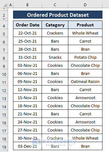
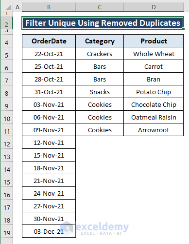
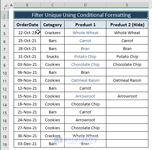
Let’s say we have three simple columns in an Excel dataset containing Order Date, Category, and Product information. We want the unique ordered products within the entire dataset.
Method 1 – Using Excel’s Remove Duplicates Feature to Filter Unique Values
Steps:
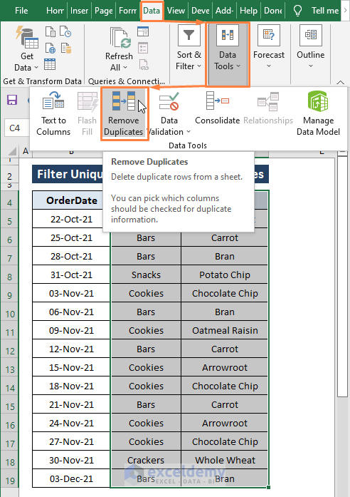
- Select the range (i.e., Category and Product).
- Go to the Data tab and select Remove Duplicates (from the Data Tools section).
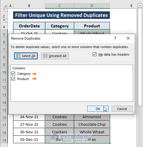
- The Remove Duplicates window appears. In the Remove Duplicates window, check all the columns.
- Tick the option My data has headers.
- Click OK.
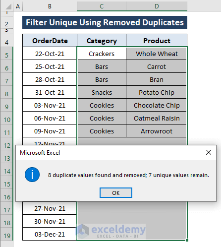
- A confirmation dialog box appears saying how many duplicate values found and removed and how many unique values remain.
- Click OK.
- The columns have been cut based on a matched pair of product and category.
Method 2 – Using Conditional Formatting to Filter Unique Values
Case 2.1 – Conditional Formatting to Filter Unique Values
Steps:
- Select the range (i.e., Product 1).
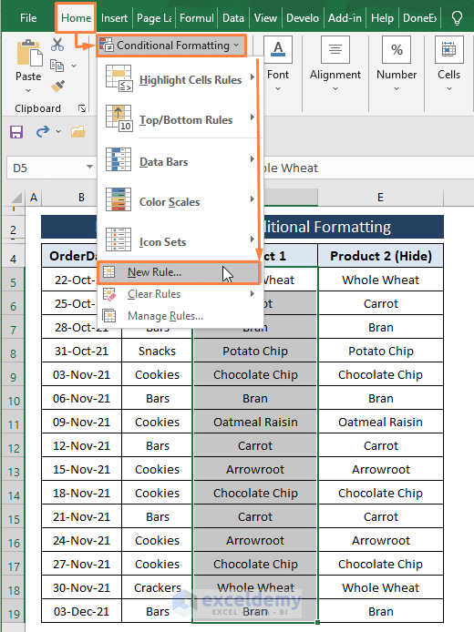
- Go to the Home tab and select Conditional Formatting (from Styles section).
- Select New Rule.
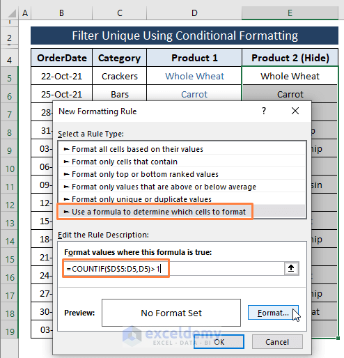
- The New Formatting Rule window pops up.
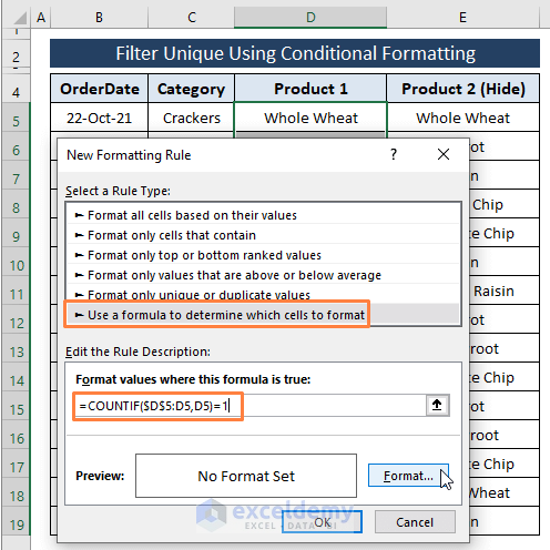
- Choose Use a formula to determine which cells to format under Select a Rule Type option.
- Copy the following formula under the Edit the Rule Description option.
=COUNTIF($D$5:D5,D5)=1In the formula, we directed Excel to count each cell in the D column as Unique (i.e., equal to 1). If the entries match with the imposed condition it returns TRUE and Color Format the cells.
- Click on Format.
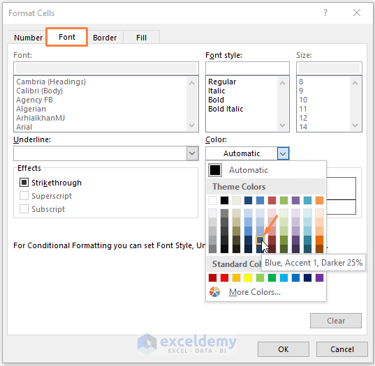
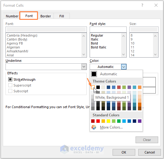
- In the Format Cells window, go to the Font section and select any formatting color as depicted in the below image.
- Click OK.
- Click OK again.

- You’ll get the unique entries color formatted.
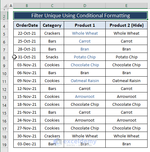
Case 2.2 – Conditional Formatting to Hide Duplicates
Steps:
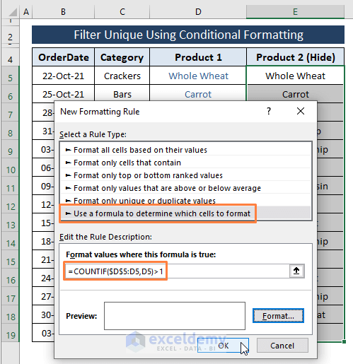
- Create a New Conditional Formatting Rule (see Case 1), but change the formula to:
=COUNTIF($D$5:D5,D5)>1The formula directs Excel to count each cell in the D column as Duplicates (i.e., greater than 1). If the entries match with the imposed condition it returns TRUE and Color Format (i.e., Hide) the cells.
- Click on Format.
- Make the Font color White.
- Click on OK.
- Click OK again.
- Here’s how the column Product 2 will look in the sample.
Method 3 – Using the Data Tab Advanced Filter Feature to Filter Unique Values
Steps:
- Select the range (i.e., Product column).
- Go to the Data tab and select Advanced from the Sort & Filter section.
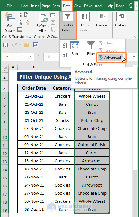
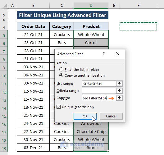
- The Advanced Filter window appears. Select Copy to another location under the Action option.
- You can choose either Filter the list, in-place, or Copy to another location. We chose the last one.
- Assign a location (i.e., F4) in the Copy to option.
- Check the Unique records only option.
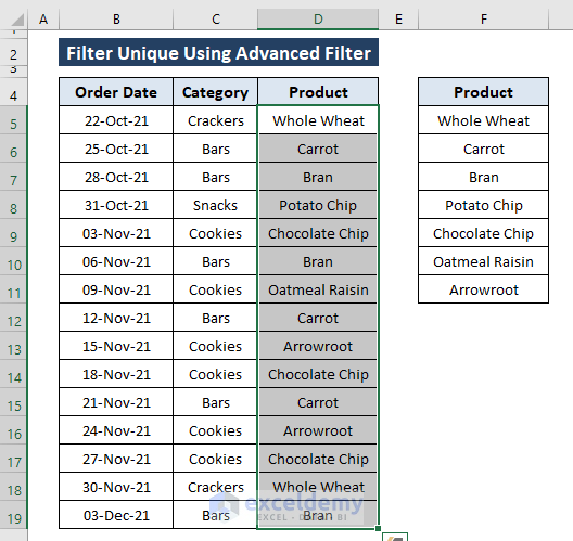
- Click OK.
- This extracts the unique values from the column into another column.
Method 4 – Filtering Unique Values Using the Excel UNIQUE Function
The UNIQUE function fetches a list of unique entries from a range or array. The syntax of the UNIQUE function is
UNIQUE (array, [by_col], [exactly_once])
The arguments,
array; range, or array from where the unique values get extracted from.
[by_col]; ways to compare and extract values, by row = FALSE (default) and by column = TRUE. [optional]
[exactly_once]; once occurring values = TRUE and existing unique values = FALSE (by default). [optional]
Steps:
- Copy the following formula in any blank cell (i.e., E5).
=UNIQUE(D5:D19)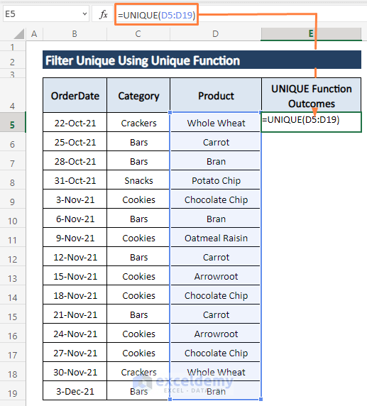
- Press Enter.
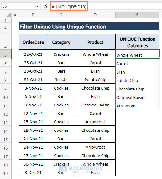
- The UNIQUE function spills all the unique entries simultaneously as an array.
The UNIQUE function only works in the Excel 365 version.
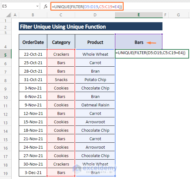
Method 5 – Using UNIQUE and FILTER Functions (with Criteria)
Let’s fetch the unique Product names of the Bars (i.e., E4) category from our dataset.
Steps:
- Use the following formula in any cell (i.e., E5).
=UNIQUE(FILTER(D5:D19,C5:C19=E4))The formula filters the D5:D19 range, imposing a condition on range C5:C19 to be equal to the cell E4.
- Hit Enter.
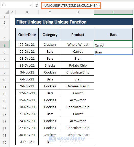
The FILTER function is only available in Excel 365.
Method 6 – Using MATCH and INDEX Functions (Array Formula)
Case 6.1 – MATCH and INDEX Functions to Filter Unique Values from a Non-Blank Range
Steps:
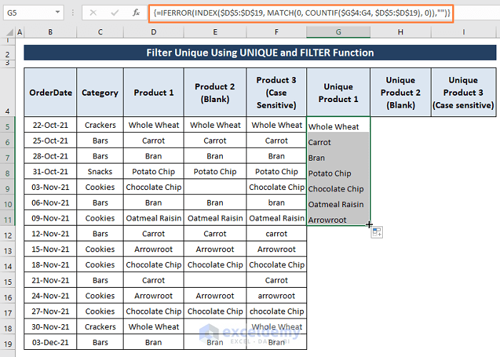
- Use the following formula in cell G5 to filter out the unique values:
=IFERROR(INDEX($D$5:$D$19, MATCH(0, COUNTIF($G$4:G4, $D$5:$D$19), 0)),"")COUNTIF($G$4:G4, $D$5:$D$19) counts the number of cells in the range (i.e., $G$4:G4) obeying the condition (i.e., $D$5:$D$19). COUNTIF returns 1 if it finds $G$4:G4 in the range. Otherwise, it returns 0.
MATCH(0, COUNTIF($G$4:G4, $D$5:$D$19), 0)) returns the relative position of a product in the range.
INDEX($D$5:$D$19, MATCH(0, COUNTIF($G$4:G4, $D$5:$D$19), 0)) returns the cell entries that meet the condition.
The IFERROR function restricts the formula from displaying any errors in outcomes.
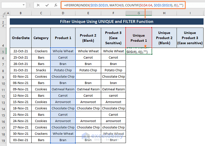
- As the formula is an array formula, press Ctrl + Shift + Enter to apply it.
Case 6.2 – MATCH and INDEX Functions to Filter Unique Values from Existing Blank Cells in a Range
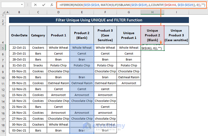
Now, in the Product 2 range, we can see multiple blank cells exist. To filter out the unique among the blank cells, we have to insert the ISBLANK function.
Steps:
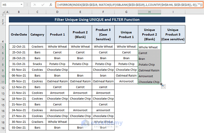
- Paste the following formula in cell H5 and press Ctrl + Shift + Enter.
=IFERROR(INDEX($E$5:$E$19, MATCH(0,IF(ISBLANK($E$5:$E$19),1,COUNTIF($H$4:H4, $E$5:$E$19)), 0)),"")This formula works in the same way as we described it in Case 6.1. However, the extra IF function with the logical test of the ISBLANK function allows the formula to ignore any blank cells in the range.
- Here’s the result of the formula.
Case 6.3 – MATCH and INDEX Functions to Filter Unique Values from a Case-Sensitive Range
Steps:
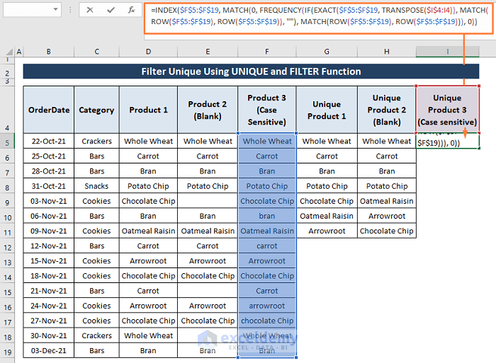
- Apply the below formula in cell I5, then press Ctrl + Shift + Enter.
=INDEX($F$5:$F$19, MATCH(0, FREQUENCY(IF(EXACT($F$5:$F$19, TRANSPOSE($I$4:I4)), MATCH(ROW($F$5:$F$19), ROW($F$5:$F$19)), ""), MATCH(ROW($F$5:$F$19), ROW($F$5:$F$19))), 0))Sections of the formula,
- TRANSPOSE($I$4:I4); transpose previous values by converting semicolon into comma. (i.e., TRANSPOSE({“unique values (case sensitive)”;Whole Wheat”}) becomes {“unique values (case sensitive)”,”Whole Wheat”}
- EXACT($F$5:$F$19, TRANSPOSE($I$4:I4); checks whether strings are the same and case-sensitive or not.
- IF(EXACT($F$5:$F$19, TRANSPOSE($I$4:I4)), MATCH(ROW($F$5:$F$19), ROW($F$5:$F$19)); returns the relative position of a string in the array if TRUE.
- FREQUENCY(IF(EXACT($F$5:$F$19, TRANSPOSE($I$4:I4)), MATCH(ROW($F$5:$F$19), ROW($F$5:$F$19)), “”); calculates how many times a string is present in the array.
- MATCH(0, FREQUENCY(IF(EXACT($F$5:$F$19, TRANSPOSE($I$4:I4)), MATCH(ROW($F$5:$F$19), ROW($F$5:$F$19)), “”), MATCH(ROW($F$5:$F$19), ROW($F$5:$F$19))), 0)); finds first False (i.e., Empty) values in the array.
- INDEX($F$5:$F$19, MATCH(0, FREQUENCY(IF(EXACT($F$5:$F$19, TRANSPOSE($I$4:I4)), MATCH(ROW($F$5:$F$19), ROW($F$5:$F$19)), “”), MATCH(ROW($F$5:$F$19), ROW($F$5:$F$19))), 0)); returns unique values from the array.
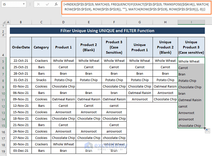
- Once you apply the formula, the case-sensitive unique values appear in the cells.
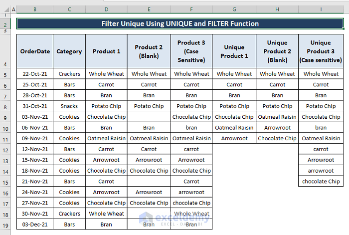
- The whole dataset looks like the below image after sorting all types of entries in their respective columns.
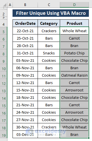
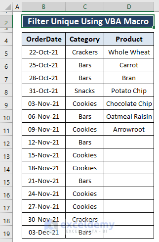
Method 7 – Using VBA Macro Code to Filter Unique Values
Consider a dataset of the following type, where we’ll use the Product column to filter unique values.
Steps:
- Press Alt + F11 to open up Microsoft Visual Basic window.
- Go to the Insert tab (in the Toolbar) and select Module.
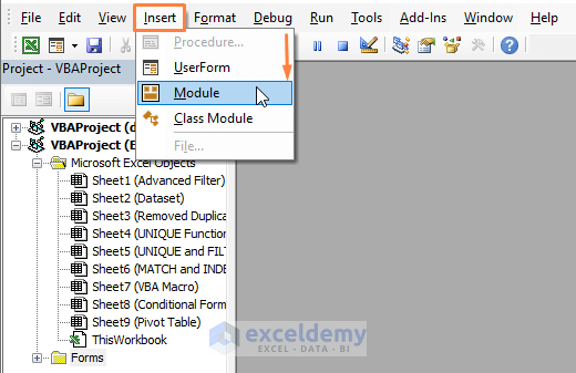
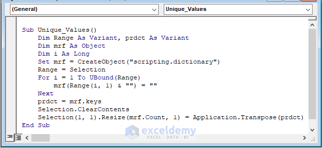
- The Module window appears. In the Module, paste the following code:
Sub Unique_Values()
Dim Range As Variant, prdct As Variant
Dim mrf As Object
Dim i As Long
Set mrf = CreateObject("scripting.dictionary")
Range = Selection
For i = 1 To UBound(Range)
mrf(Range(i, 1) & "") = ""
Next
prdct = mrf.keys
Selection.ClearContents
Selection(1, 1).Resize(mrf.Count, 1) = Application.Transpose(prdct)
End Sub
mrf = CreateObject(“scripting.dictionary”) creates an object that is assigned to mrf.
Selection assigned to the Range. The For loop takes each cell and then matches it with the Range for duplicates. The code clears the Selection and fills it with unique values.
- Hit F5 to run the macro.
- Return to the worksheet and you see all the unique values from the selection.
Method 8 – Using a Pivot Table to Filter Unique Values
Steps:
- Select a range you want to filter.
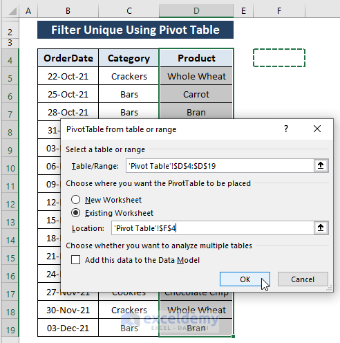
- Go to the Insert tab and select PivotTable from the Tables section.
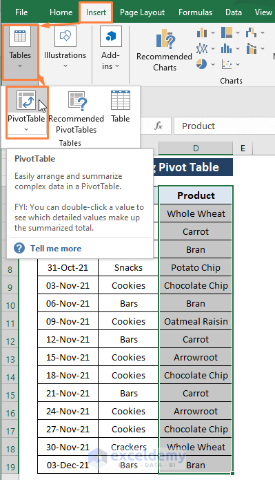
- The PivotTable from a table or range window appears. The range (i.e., D4:D19) will be automatically selected.
- Choose Existing Worksheet for the where you want the PivotTable to be placed option.
- Click OK.
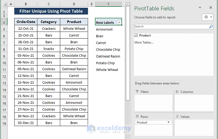
- The PivotTable Fields window appears. There is only one field (i.e., Product).
- Check the Product field to make the unique product list appear as shown in the picture below.
Download the Excel Workbook
<< Go Back to Filter in Excel | Learn Excel
Get FREE Advanced Excel Exercises with Solutions!
