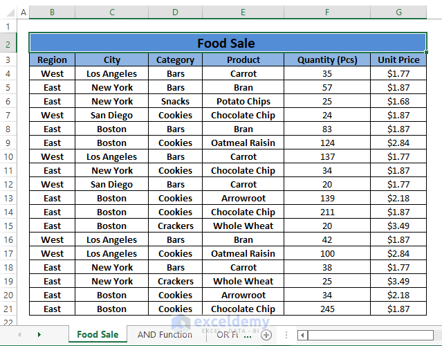
Consider a dataset of Product Sales, where we have text value columns named Region, City, Category, and Product. We want to conditionally format the dataset depending on the multiple text values of these text value columns.
Conditional Formatting for Multiple Text Values in Excel: 4 Easy Ways
Method 1 – Using the AND Function
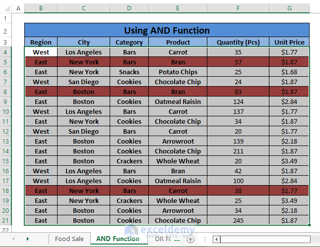
We have four text columns to which we want to highlight the rows which have “East” as Region and “Bars” as Category.
Steps:
- Select the entire range ($B$4:$G$21) you want to format.
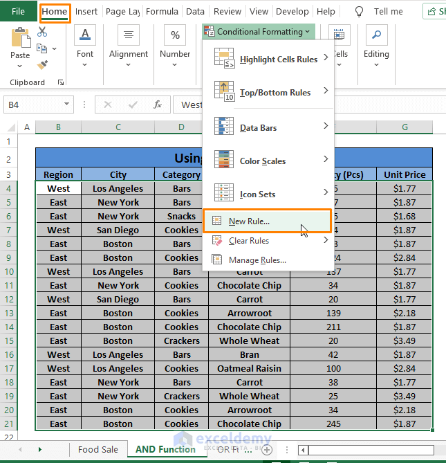
- Go to the Home tab and select Conditional Formatting (in the Styles section).
- Select New Rule (from the drop-down options).
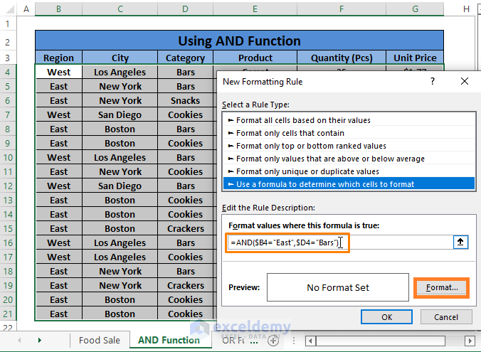
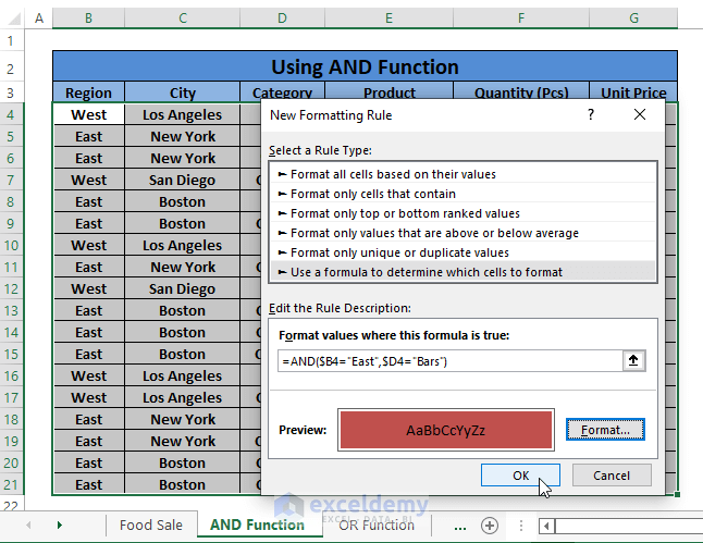
- A New Formatting Rule window pops up. Select Use a formula to determine which cell to format (from Select a Rule Type dialog box).
- Paste the following formula in the Edit the Rule Description box:
=AND($B4="East",$D4="Bars")The syntax of the AND function is
AND(logical1,[logical2]...)Inside the formula,
$B4=”East”; is the logical1 argument.
$D4=”Bars“; is the logical2 argument.
The formula formats the rows for which these two arguments are True.
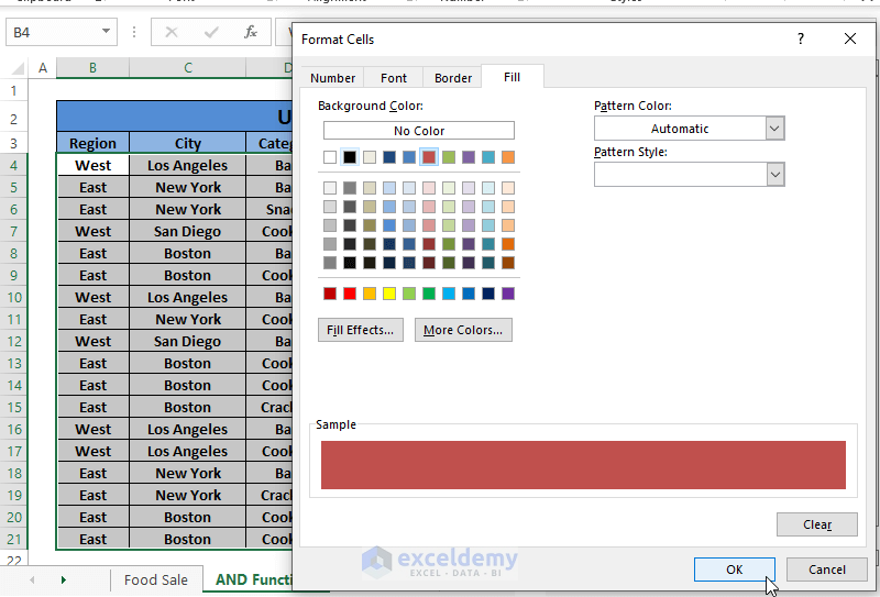
- Click on Format. The Format Cells window opens.
- From the Format Cells window, choose any Fill color from the Fill section.
- Click OK.
- You’ll return to the New Formatting Rule dialog box. Click OK.
- All the matching rows in the dataset get formatted with the fill color we selected.
Read more: How to Change a Row Color Based on a Text Value in a Cell in Excel
Method 2 – Using the OR Function
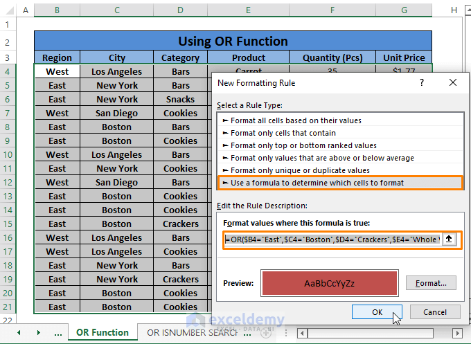
We want to format rows which have any of the entries: “East”, “Boston”, “Crackers”, and “Whole Wheat”.
Steps:
- Repeat the Steps from Method 1. Replace the formula in Edit the Rule Description with the following:
=OR($B4="East",$C4="Boston",$D4="Crackers",$E4="Whole Wheat")Here, we have checked whether B4, C4, D4, and E4 cells are equal to “East”, “Boston”, “Crackers”, and “Whole Wheat” respectively. OR will trigger the action if any of the conditions match.
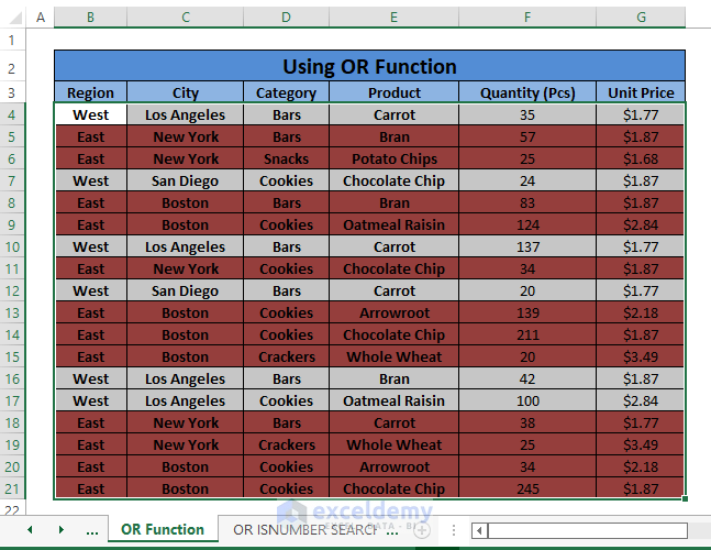
- You’ll see the formula formats all the rows that contain any of the text we mentioned earlier.
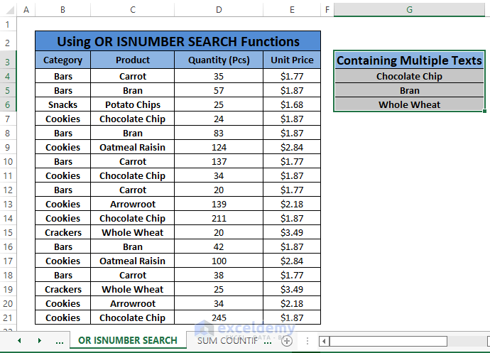
Method 3 – Using OR, ISNUMBER, and SEARCH Functions
We have multiple products such as Chocolate Chip, Bran, and Whole Wheat. We want to highlight all the rows that contain these certain Products.
Steps:
- Insert the names of the Products in a new column (i.e., Containing Multiple Texts).
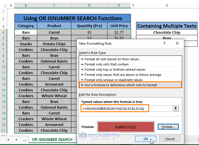
- Repeat the Steps from Method 1. Replace the formula in Format values where the formula is true dialog box with the following:
=OR(ISNUMBER(SEARCH($G$4:$G$7,$C4)))Inside the formula,
The SEARCH function matches texts existing in the Range $G$4:$G$7 to the lookup Range starting cell $C4. Then the ISNUMBER function returns the values as True or False. In the end, the OR function matches alternating any of the text within the find_value Range (i.e.,$G$4:$G$7).
- The inserted formula formats all the rows in the dataset matching the texts with the Containing Multiple Texts columns.
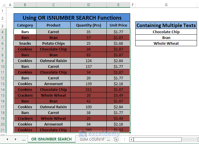
Make sure you select the particular Range ($G$4:$G$7) as find_text inside the SEARCH function.
Read more: How to Do Conditional Formatting for Multiple Conditions
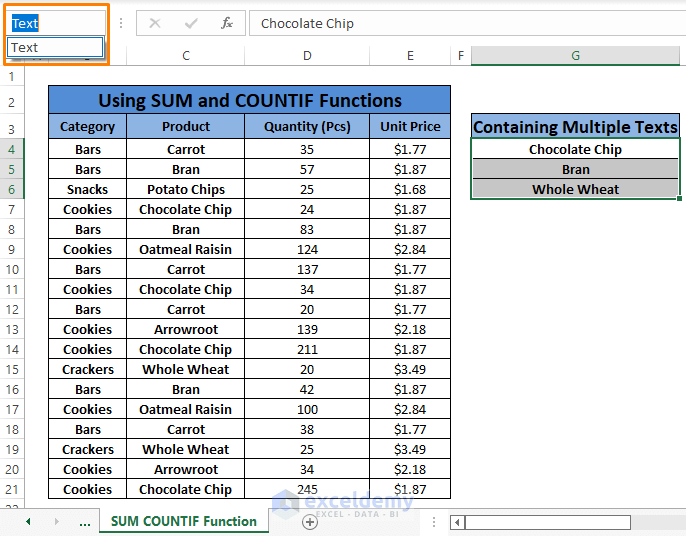
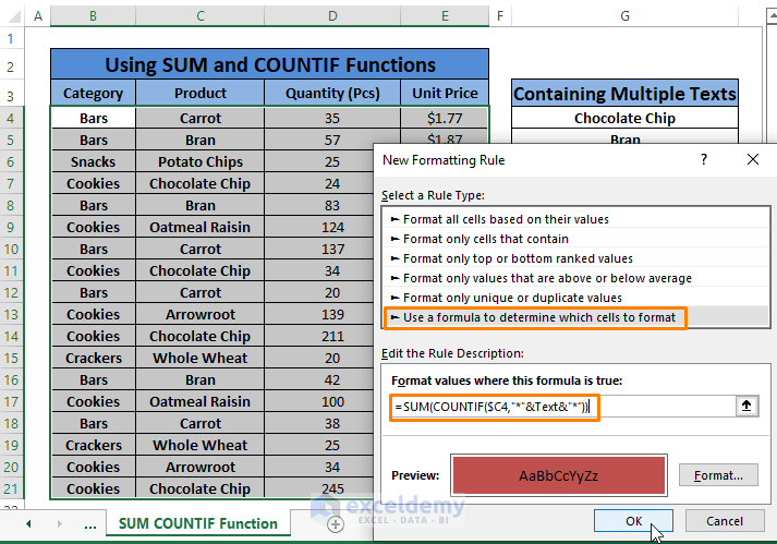
Method 4 – Using the SUM and COUNTIF Functions
Steps:
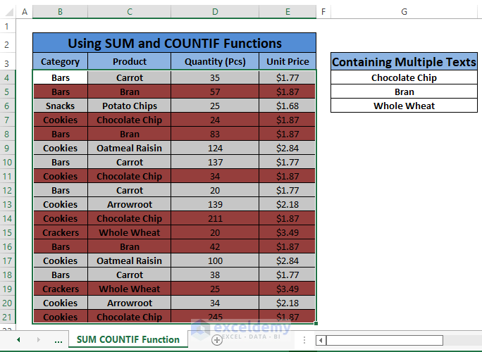
- Assign a name (i.e., Text) to all the Products in the Containing Multiple Texts columns.
- Repeat the Steps from Method 1. Replace the formula for formatting with the formula below:
=SUM(COUNTIF($C4,"*"&Text&"*"))In the formula,
The COUNTIF matches only one criterion (i.e., Chocolate Chip) to the Range starting from the cell $C4. Combining the COUNTIF function with the SUM function enables it to match all the criteria (i.e., Text) to the Range.
- The formula formats all the rows containing texts that match with the assigned name Texts.
Practice Dataset for Download
Further Readings
- How to Format Cell Based on Formula in Excel
- How to Use Conditional Formatting Based on VLOOKUP in Excel
- How to Apply Conditional Formatting with INDEX-MATCH in Excel
- Excel Conditional Formatting Formula with IF
- Excel Conditional Formatting Formula If Cell Contains Text
- Conditional Formatting If Cell is Not Blank
- How to Change Text Color Based on Value with Excel Formula
- Conditional Formatting Entire Column Based on Another Column in Excel
- Excel Highlight Cell If Value Greater Than Another Cell
<< Go Back to Conditional Formatting with Multiple Conditions | Conditional Formatting | Learn Excel
Get FREE Advanced Excel Exercises with Solutions!

Hi i have a problem if containing multiple texts columns have empty cells how to exclude them.
You can exclude or ignore the blanks using 2 simple tricks.
1. Use an additional formula in conditional formatting. Go to conditional formatting > New Rule option > select Format Only Cell that contains rule type > Select Blanks from edit rule description > Keep Cell format as no cell format. Click OK.
2. Go to Conditional formatting > New Rule option> Select Use a formula to determine which cell to format rule type > type “=ISBLANK(Cell Reference)=TRUE” in the Edit the Rule description box > Keep Cell format as no cell format. Click OK.
Hope these tricks work for you.
Wow, what a write up. Wish the author would have wrote an article that pertained to the title. This article needs to be titled “Using Conditional Formatting to Highlight ROWS Based on Multiple Cell Vallues.”
Hello Shane V,
Thank you for sharing your thoughts! If you change the “Apply to” selection in the conditional formatting rules, you can target individual cells or columns, not just rows. This makes it possible to highlight multiple text values in any range, not only across entire rows. Hope this helps!
Regards
ExcelDemy
Hi, just wondering how to write a conditional formatting rule for the following example.
I have a spreadsheet and in $F2 there are 4 choices in a drop down list.
Value 1 = Blue
Value 2 = Red
Value 3 = Green
Value 4 = Yellow.
If either value (Red or Green) is selected, then the formatting will apply to the row, the formatting is the same for each of those 2 choices.
I have one that works when a single value is selected but not sure how to broaden it. (eg – rule is applied to $A2:$J2000 — =$F2=”Blue”). Hope you can help, many thanks
Hello DebbieV,
You can apply conditional formatting to highlight the entire row based on multiple values in your dropdown. In your case, if either “Red” or “Green” is selected in column F, you want the formatting to apply to the row.
1. Select the range you want to format (for example, A2:J2000).
2. Go to Home tab >> select Conditional Formatting >> select New Rule.
3. Select Use a formula to determine which cells to format.
4. Enter the following formula:
=OR($F2=”Red”, $F2=”Green”)
5. Set your desired formatting and click OK.
This rule will apply the formatting to the entire row whenever Red or Green is selected in column F.
Regards
ExcelDemy