Method 1 – Calculate the Area Under the Curve with the Trapezoidal Rule in Excel
It is not possible to directly calculate the area under the curve. We can break the whole curve into trapezoids. By adding the areas of the trapezoids, we can get the total area under the curve.
STEPS:
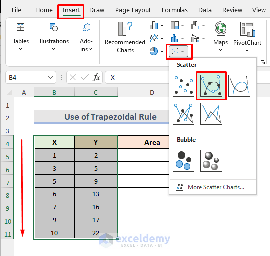
- Select the range B4:C11 from the dataset.
- Go to the Insert tab.
- Select the Insert Scatter (X, Y) option from the Charts section.
- From the drop-down, select Scatter with Smooth Lines and Markers option.
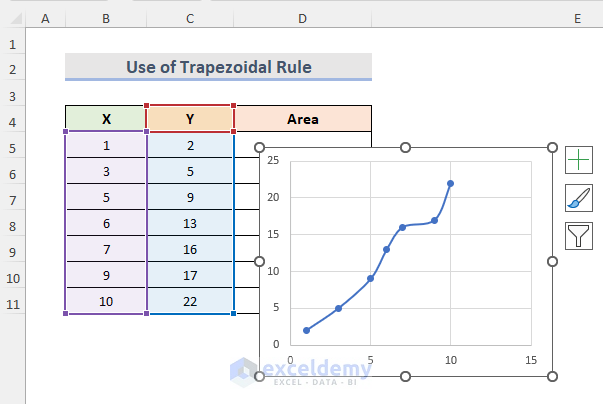
This will open a chart like the one below.
- Calculate the area of the trapezoid which is between X = 1 & X = 3 under the curve by entering the following formula in cell D5:
=((C5+C6)/2)*(B6-B5)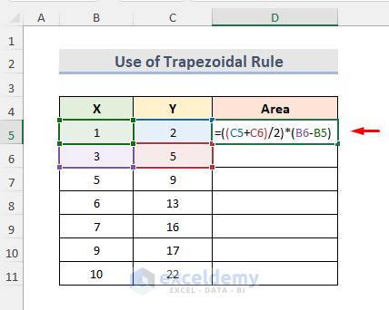
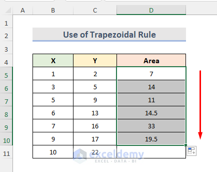
- Press Enter.
- Use the Fill Handle tool till the second last cell to get the area of the trapezoids.
- Add all the areas of the trapezoids by entering the following formula in cell D13.
=SUM(D5:D10)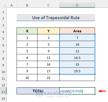
We have used the SUM function to add up the cell range D5:D10.
- Press Enter to see the result.

Method 2 – Use Excel Chart Trendline to Get Area Under Curve
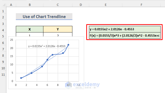
Excel Chart Trendline helps us to find an equation for the curve. We use this equation to get the area under the curve. Suppose, we have the same dataset containing different points on the X & Y axes in columns B & C respectively. We will use the chart trendline to get the equation from which we can get the area under the curve.
STEPS:
- Select the chart.
Select the range B4:C11 > go to Insert tab > select Insert Scatter (X, Y) from the drop-down > select Scatter with Smooth Lines and Markers option.
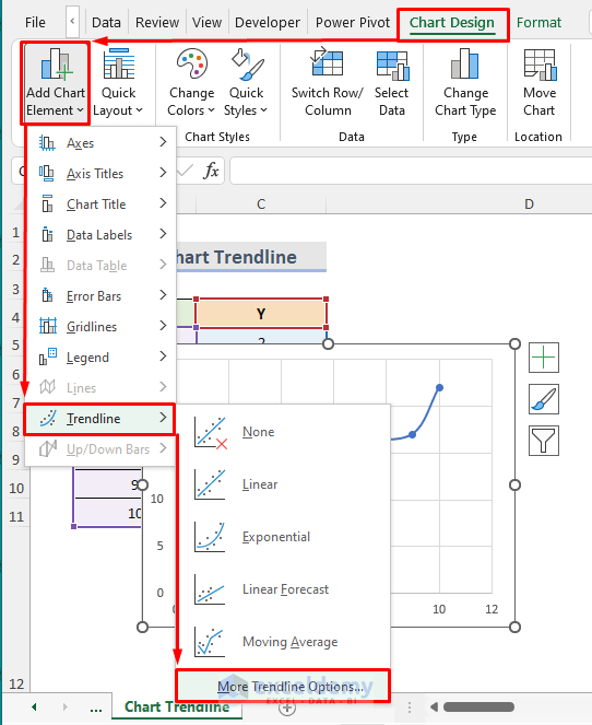
- Go to the Chart Design tab.
- Select Add Chart Element drop-down from the Chart Layouts section.
- From the drop-down, go to the Trendline option.
- Select More Trendline Options.
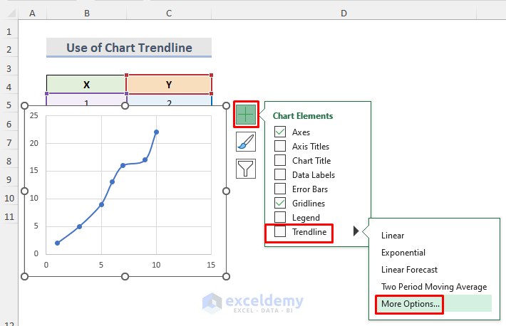
- Or you can simply click on the Plus (+) sign on the right side of the chart after selecting it.
- This will open the Chart Elements section.
- From that section, place the cursor over the Trendline section and click on More Options.
- In the Format Trendline window, select Polynomial from the Trendline Options.
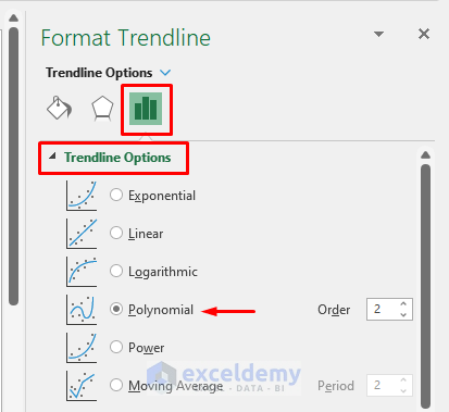
- Check the Display Equation on chart option.
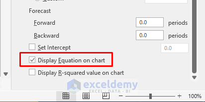
The polynomial equation will be displayed on the chart.
- The polynomial equation is:
y = 0.0155×2 + 2.0126x – 0.4553
- We need to get the definite integral of this polynomial equation which is:
F(x) = (0.0155/3)x^3 + (2.0126/2)x^2 – 0.4553x+c
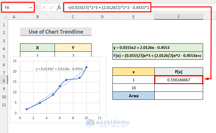
- We will put the value x = 1 in the definite integral. We can see the below calculation in cell F8:
F(1) = (0.0155/3)*1^3 + (2.0126/2)*1^2 - 0.4553*1- Press Enter to see the result.
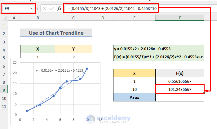
- We will enter x = 10 in the definite integral. The calculation will be like the following in cell F9:
F(10) =(0.0155/3)*10^3 + (2.0126/2)*10^2 - 0.4553*10- Press Enter to see the result.
- We will calculate the difference between the calculations of F(1) & F(10) to find the area under the curve.
- Enter the following formula in cell F10.
=F9-F8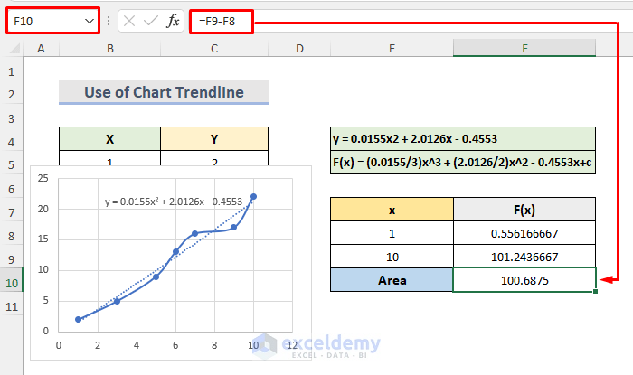
- Press Enter to see the result.
Practice Workbook
<< Go Back to Formula List | Learn Excel
Get FREE Advanced Excel Exercises with Solutions!
