Method 1 – Using Filter Feature to Delete Every Other Row in Excel
Step 1:
- Select the column header. From your Home Tab, go to the Editing Ribbon and select Sort & Filter.
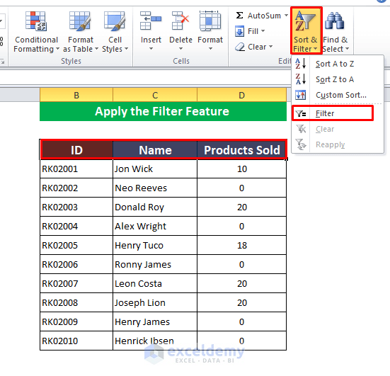
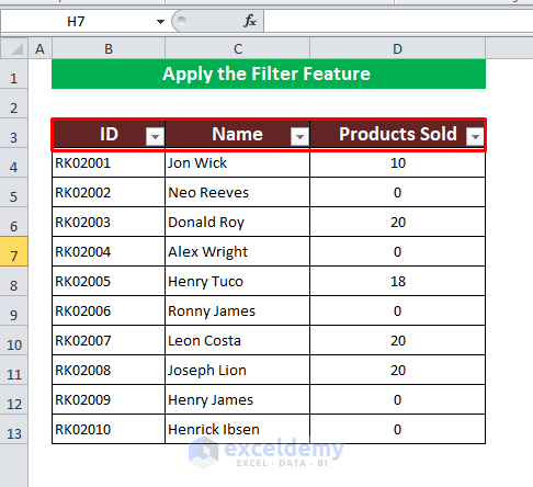
- Each column header now has a filter icon.
Step 2:
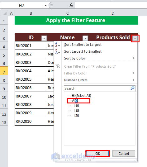
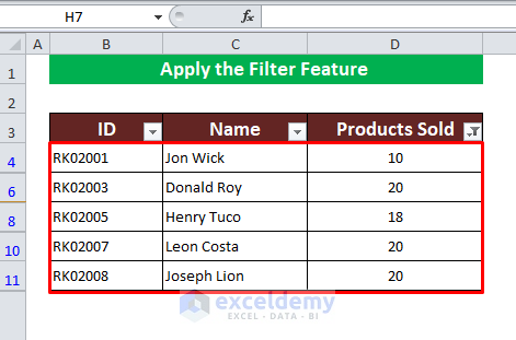
- Delete those rows that do not have Zero Products Sold.
- Select the Products Sold column and click the Drop-Down icon in the column.
- Select Zero to keep it and filter out the rest.
- Click OK to continue.
- The Filter command deletes every other row.

- You can also keep all the rows without zero values and delete rows that have zeros. Open the Filter option, select the zero option, and select the rest.
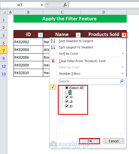
- Using the Filter feature, you can delete every other row in Excel.
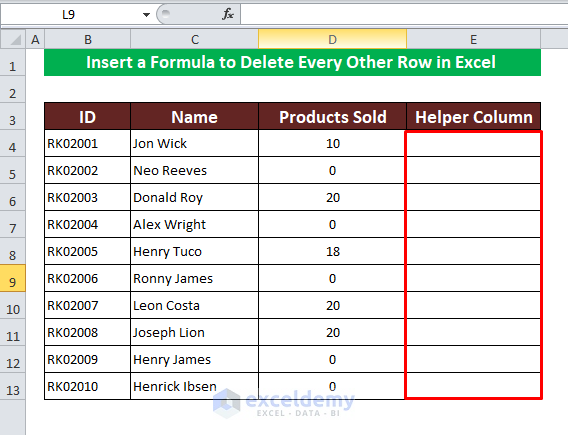
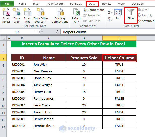
Method 2 – Inserting ISEVEN and ROW Functions to Delete Every Other Row
Step 1:
- You need a Helper Column to apply the formula.
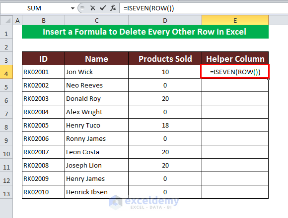
Step 2:
- In Cell E4 of the Helper Column, apply the ISEVEN with the ROW. The formula is:
=ISEVEN(ROW())- This formula will return TRUE for all EVEN rows and FALSE for all ODD.
- Press Enter.
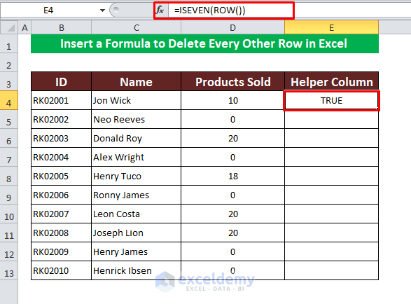
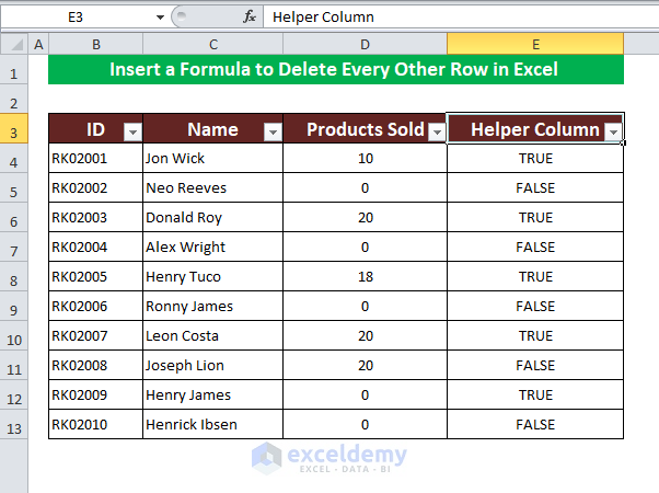
- Apply the formula to the rest of the cells.

Step 3:
- Filter out the true or false values. Select your column header; go to Data Tab, and click on Filter from Sort & Filter Ribbon to apply the filter option.
- You added a filter option to every column.
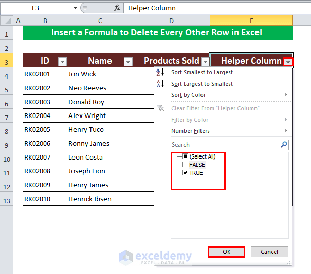
- If you need to delete the even rows, open the filter option, select TRUE to keep those even rows and filter every other row. Click OK to proceed.
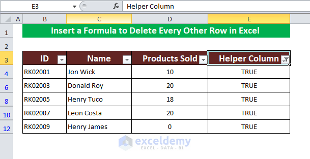
- Only the even rows remained.
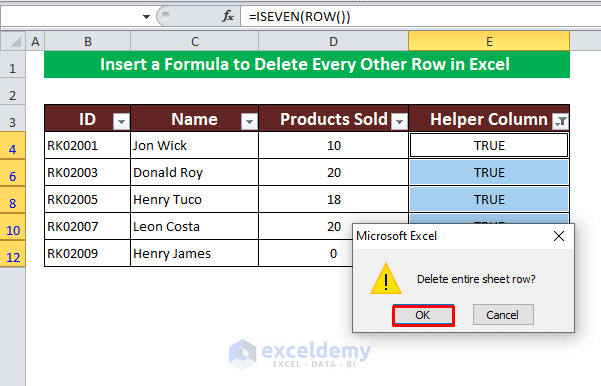
- Select then all and right-click on the mouse to open options. Choose Delete Row.
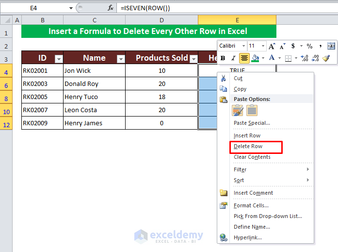
- A warning message box appears. Click OK to confirm.
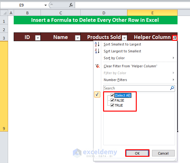
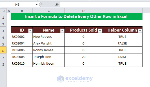
- The dataset is blank now. Click the Helper Column‘s drop-down icon. Select FALSE to restore those rows.
- There are only ODD rows in the dataset.
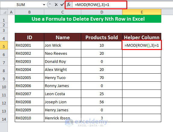
Method 3 – Use MOD and ROW Functions to Delete Every Nth Row in Excel
Step 1:
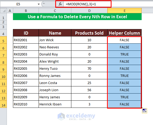
- In Cell E5, apply the MOD function with the ROW. The formula is:
=MOD(ROW(),3)=1- This formula returns TRUE for every third row and FALSE for every other.
- Enter to get the result. Apply the same formula to the rest of the cells.
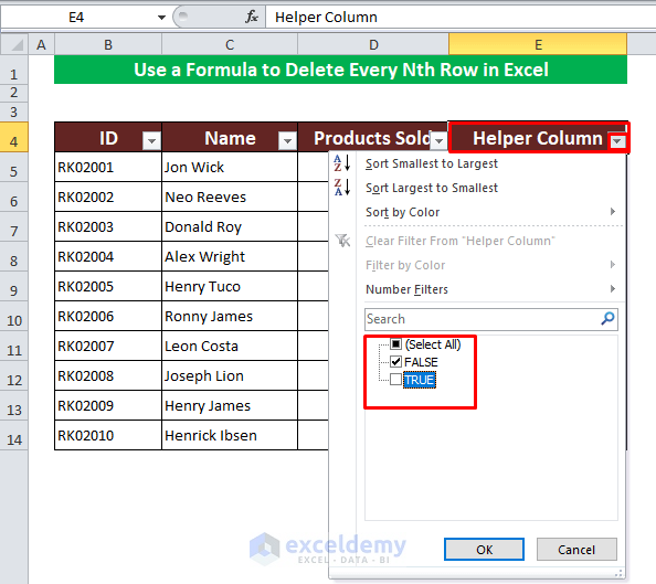
Step 2:
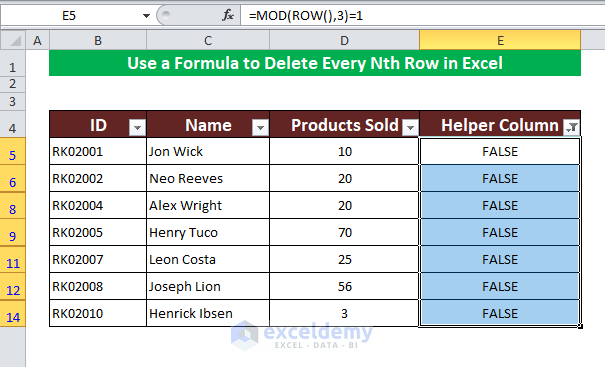
- Delete every third row here. Add the filter option to your column header, and from the option, select FALSE to keep them and delete every other row.
- Our task is complete.
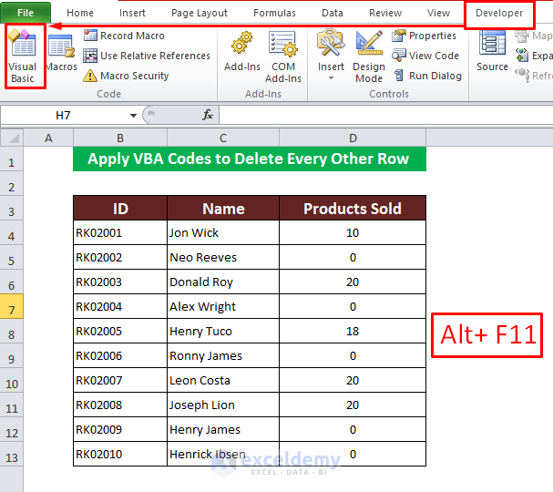
Method 4 – Applying Excel VBA Codes to Delete Every Other Row
Step 1:
- Go to the Developer Tab and click on Visual Basic to open the VBA. Alternatively, you can press Alt+F11 to open it.
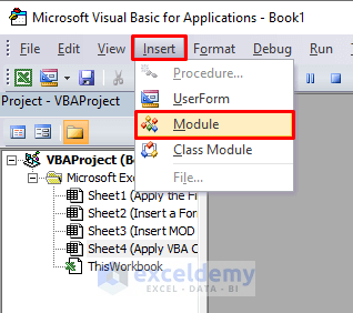
- Click Insert in the VBA window, and from the option select Module to insert one.
Step 2:
- Write the code by copying and pasting it. This code will delete every second row from your dataset.
Sub DeleteEveryOtherRow()
'Delete Row
Dim rng As Range
Dim InputRng As Range
xTitleId = "Delete Row Using VBA"
Set InputRng = Application.Selection
Set InputRng = Application.InputBox("Range :", xTitleId, InputRng.Address, Type:=8)
Application.ScreenUpdating = False
For i = InputRng.Rows.Count To 1 Step -2
            Set rng = InputRng.Cells(i, 1)
    rng.EntireRow.Delete
Next
Application.ScreenUpdating = True
End Sub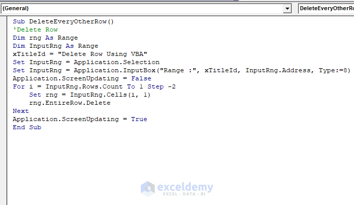
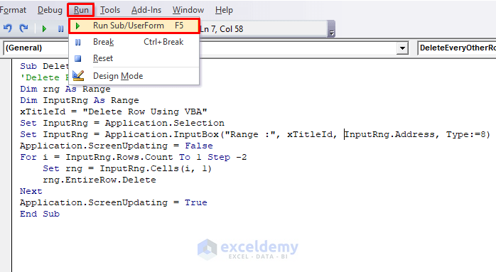
- Click Run to run the code, or press F5.
Step 3:
- Select the dataset from the worksheet ($B$4:$D$13).
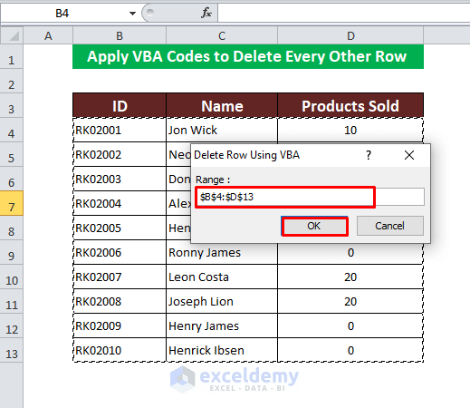
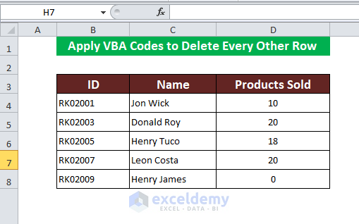
- Click OK, and every second row will be deleted from the dataset.
Things to Remember
The MOD with the ROW formula will return FALSE to every third row from the main worksheet.
The VBA code provided in this article will delete every second row from the dataset.
Download Practice Workbook
Download this practice book to exercise the task while reading this article.
Related Article
<< Go Back to Delete Rows | Rows in Excel | Learn Excel
Get FREE Advanced Excel Exercises with Solutions!
