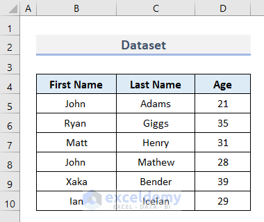
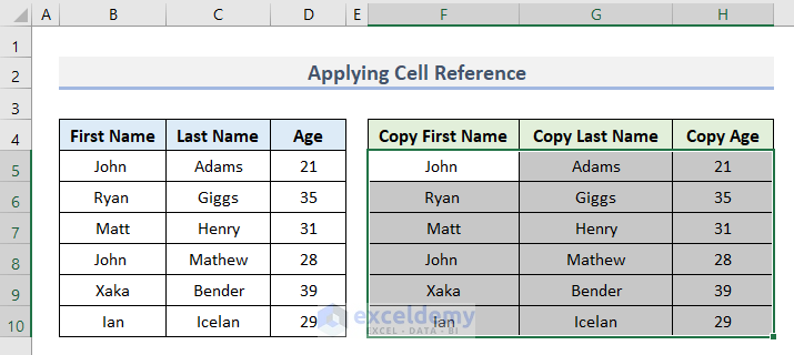
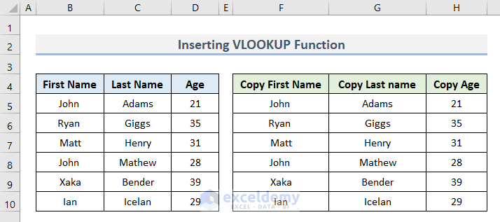
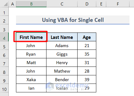
In this dataset, there are five people’s First Names, Last Names and Ages. Using Excel formulas, we will copy cell value from this dataset to another cell.
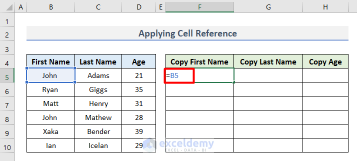
Method 1 – Copy Cell Value to Another Cell Using Cell Reference in Excel
- Select cell F5 and type this formula to extract the value of cell B5:
=B5- Hit Enter.
- Apply the same process in cell G5 with this formula.
=C5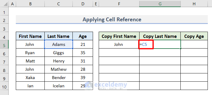
- Copy the value of cell D5 to cell H5 with this formula.
=D5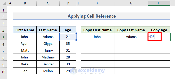
- Select the cell range F5:H5 and use the Autofill tool to copy the rest of the values from the dataset all at once.
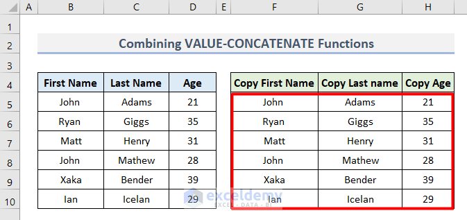
Method 2 – Combining VALUE-CONCATENATE Functions to Copy Cell Value to Another
- Insert this formula in cell F5:
=IFERROR(VALUE(B5),CONCATENATE(B5))- Press Enter.
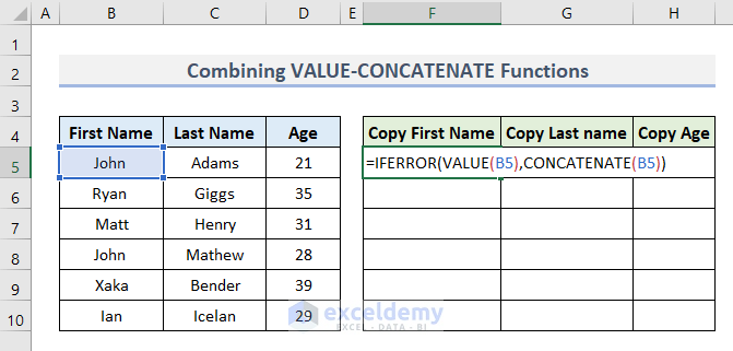
In this formula, the CONCATENATE function is used to add strings together of cell B5. then we used the VALUE function to extract numerical values if any. Lastly, use the IFERROR function to avoid any sort of error in the calculation.
- Apply a similar procedure in cell G5:
=IFERROR(VALUE(C5),CONCATENATE(C5))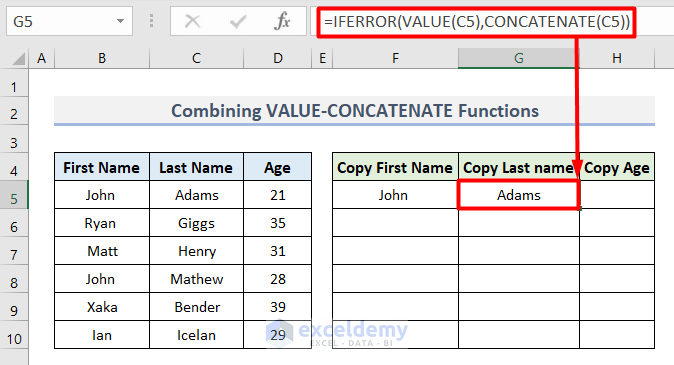
- Use this formula in cell H5.
=IFERROR(VALUE(D5),CONCATENATE(D5))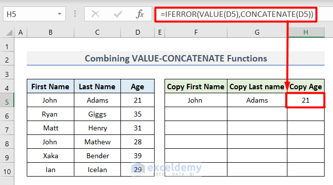
- Go through the same procedure for cell range F6:H10 and you will get the following output.
Note: You cannot use the CONCATENATE or the VALUE functions individually for this process, because one extracts text string and the other one extracts numbers. This is why you need to combine them to get a wholesome solution for any kind of value.
Method 3 – Copying Cell Value with Excel VLOOKUP Function
- Insert this formula to extract the cell value of B5 to cell F5, then hit Enter:
=VLOOKUP(B5,B5,1,FALSE)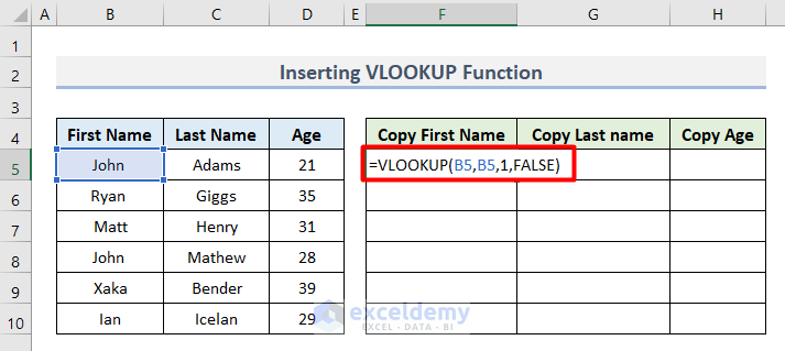
- Write the same formula for the first row of the Last Name column, changing the Cell Reference values.
=VLOOKUP(C5,C5,1,FALSE)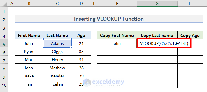
- Apply this formula in cell H5:
=VLOOKUP(D5,D5,1,FALSE)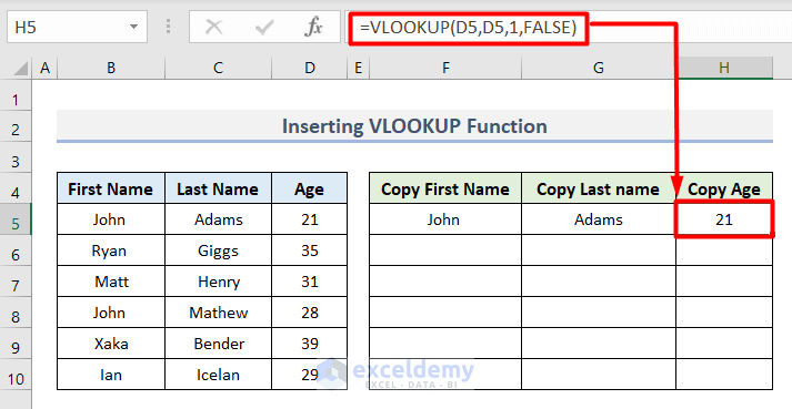
Here, the VLOOKUP function is used to set the column of the range to look for the value. Since our value will be at the start of our range, we are using 1. Then for an exact match, we wrote FALSE or 0.
- Do the same for the rest of the cells to get this final output.
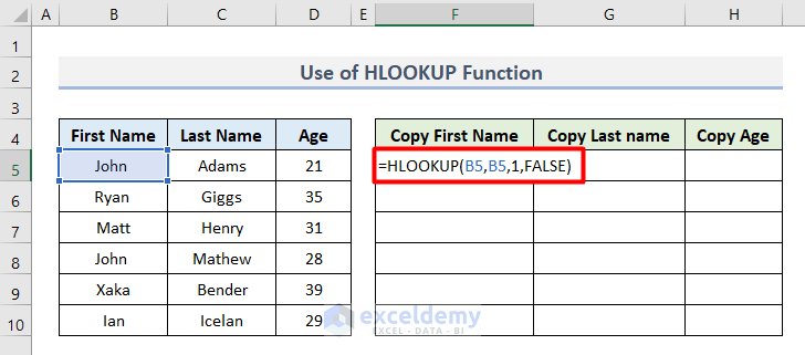
Method 4 – Copy Cell Value with HLOOKUP Function
- Type this formula in cell F5:
=HLOOKUP(B5,B5,1,FALSE)- Hit Enter.
- Apply the same formula for the rest of the cells changing the cell reference.
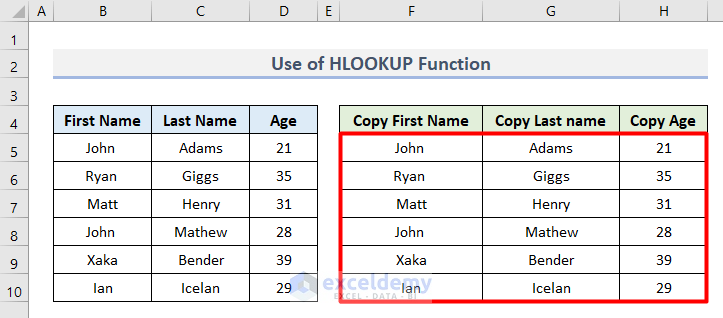
In this formula, the HLOOKUP function is used to set the column of the range to look for the value, since our value will be at the start of our range we are using 1. For an exact match, we typed FALSE.
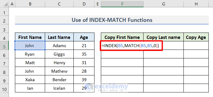
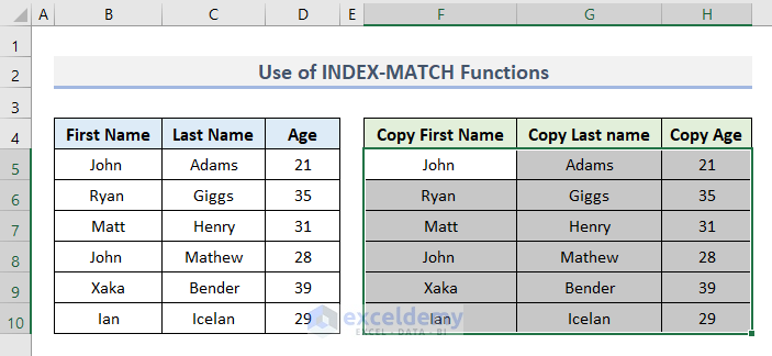
Method 5 – Excel Formula with INDEX-MATCH Functions to Copy Cell Value
- Insert this formula in cell F5 to copy the value of cell B5:
=INDEX(B5,MATCH(B5,B5,0))- Press Enter.
- Apply the same in cell G5.
=INDEX(C5,MATCH(C5,C5,0))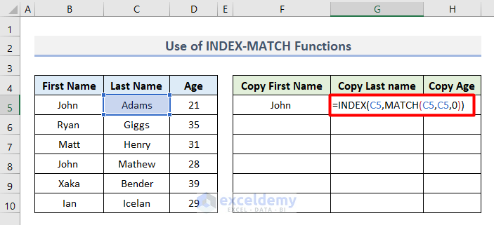
- Type a similar formula in cell H5 changing cell reference to D5:
=INDEX(D5,MATCH(D5,D5,0))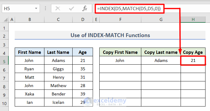
In this formula, the INDEX-MATCH functions work as a dynamic array to look for the specific value both horizontally and vertically. Along with it, type 0 for the last argument for an exact match.
- Select cell range F5:H5 and use the AutoFill tool to get this final output.
How to Copy Cell Value to Another Cell in Excel: Conventional Methods
Method 1 – Select Copy & Paste Options
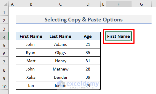
- Select cell B4.
- On the Clipboard section of the Home tab, click on Copy.
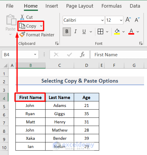
- Select the destination cell F4.
- In the Clipboard section, you will find an option called Paste.
- Click on the Paste icon from the list of options.
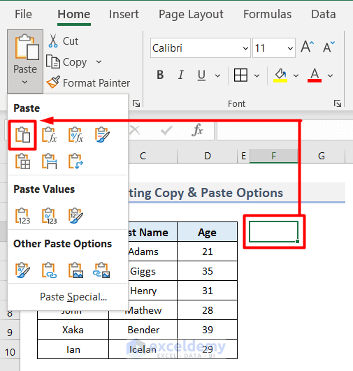
- You will get the copied value.
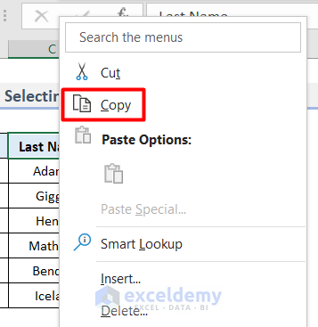
- You can get the Copy command by right-clicking on the source cell.
- Right-click on the destination cell and you will find the Paste command.
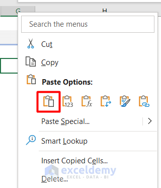
- You can try any of the copy-and-paste options.
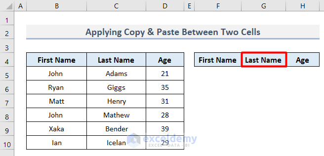
Method 2 – Copy & Paste Between Two Cells
- We copied and pasted the First Name and Age to two adjacent cells.
- Select and copy the cell having the title Last Name.
- Put the cursor to the right of most of the two adjacent cells and then right-click.
- Click on Insert Copied Cells.
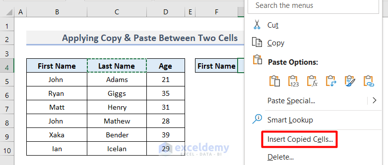
- The Insert dialogue box will open.
- Select Shift cells right and click OK.
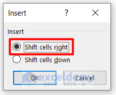
- The value will be copied between two cells.
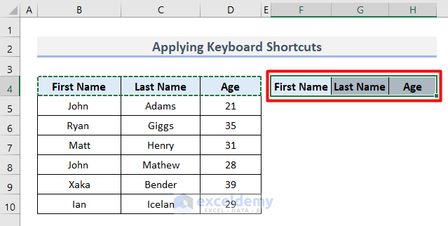
Method 3 – Apply Keyboard Shortcuts
- Select the cell range B5:D5.
- Hit Ctrl + C on your keyboard to copy the cells.

- Go to the destination cell and hit Ctrl + V to get the copied values.
How to Copy Value to Another Cell with Excel VBA
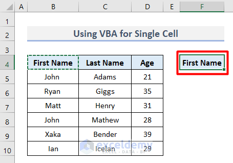
Method 1 – Copy a Single Cell
- Select cell B4 as we want to copy it.
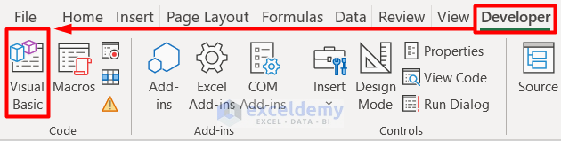
- Inside the Developer tab, select the Visual Basic option under the Code group.
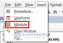
- Under the Insert option, select Module.
- Write this code here:
Sub Copy_SingleCell()

    Selection.Copy
    ActiveCell.Offset(0, 4).Range("A1").Select
    ActiveSheet.Paste
End Sub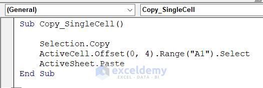
This code will select the cell and paste it at a difference of 4 columns because we have set the Offset value 0 and 4. 0 indicates no change of row, and 4 indicates the change of 4 columns. You can increase or decrease the value as you preferred.
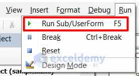
- Click on the Run Sub icon or press F5 on your keyboard.
- The code copies the cell and pastes at an offset of 4 cells column-wise.
Note: To copy the value only (not format) you can apply this code:
Sub Copy_SingleCell()
Selection.Copy
ActiveCell.Offset(0, 4).Range("A1").Select
Selection.PasteSpecial Paste:=xlPasteValues, Operation:=xlNone, SkipBlanks _
:=False, Transpose:=False
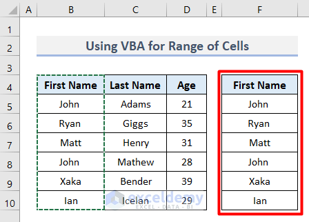
End SubMethod 2 – Copy a Range of Cells
If you want to copy a range of cells, then the code will be as follows:
Sub Copy_Range()

    Range(Selection, Selection.End(xlDown)).Select
    Selection.Copy
    ActiveCell.Offset(0, 4).Range("A1").Select
    ActiveSheet.Paste
End Sub
Finally, you will find something similar to the image below.
Additional Tips
If you want to copy a cell from another sheet all you need to do is insert the sheet name before the cell reference. For example, we wanted to get the value belonging to cell B4 of the INDEX-MATCH sheet. therefore, the formula provides this solution.
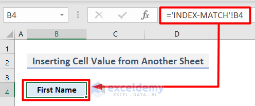
Note: When you name your sheet with multiple words you need to mention the name within an Apostrophe (
'') but for a single word name, this punctuation mark is not needed.Download Practice Workbook
You are welcome to download the workbook from the link below.
<< Go Back to Copy Cell Value | Formula List | Learn Excel
Get FREE Advanced Excel Exercises with Solutions!

I’ve been looking forever for a formula to copy the content of one cell into another one , but with no luck , until I found this page . Thank you , amazing content and so easy to understand it . You are doing an amazing job !!
Hi Alexa,
Thanks for your feedback.
Best regards
i don’t want to do it for one cell and then copy formula manually to another
imagine u have dataset 1000×1000 (u dont want to do it manually waste of nerves and time)
doesn’t work for chosen value in another cell like this with substitute value based on N5
for example
=INDEX(C:C=N5;MATCH(C:C=N5;C:C=N5;0)) – C…column date format populated
excel has stupid logic, most of functions doesn’t allow to operate like this
Hello, AHMED!
Thank you for your query. Regarding your query, you can use an array formula to accomplish this result.
Thus, all the cell values will be copied to all the desired cells in an instant.
I hope this solves your problem.
Regards,
Tanjim Reza